Way back in the mists of time, we did a little bit of work on "emergent constraints". This is a slightly hackneyed term referring to the use of a correlation across an ensemble of models between something we can’t measure but want to estimate (like the equilibrium climate sensitivity S) and something that we can measure like, say, the temperature change T that took place at the Last Glacial Maximum….
Actually our early work on this sort of stuff dates back 15 years but it was a bit more recently, in 2012 when we published this result
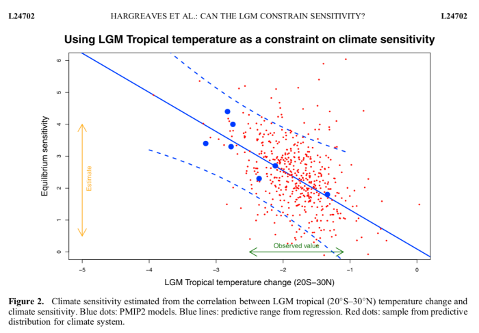
in the paper blogged about here that we started to think about it a little more carefully. It is easy to plot S against T and do a linear regression, but what does it really mean and how should the uncertainties be handled? Should we regress S on T or T on S? [I hate the arcane terminology of linear regression, the point is whether S is used to predict T (with some uncertainty) or T is used to predict S (with a different uncertainty)]. We settled for the conventional approach in the above picture, but it wasn’t entirely clear that this was best.
And is this regression-based approach better or worse than, or even much the same as, using a more conventional and well-established Bayesian Model Averaging/Weighting approach anyway? We raised these questions in the 2012 paper and I’d always intended to think about it more carefully but the opportunity never really arose until our trip to Stockholm where we met a very bright PhD student who was interested in paleoclimate stuff and shortly afterwards attended this workshop (jules helped to organise this: I don’t think I ever got round to blogging it for some reason). With the new PMIP4/CMIP6 model simulations being performed, it seemed a good time to revisit any past-future relationships and this prompted us to reconsider the underlying theory which has until now remained largely absent from the literature.
So, what is new our big idea? Well, we approached it from the principles of Bayesian updating. If you want to generate an estimate of S that is informed by the (paleoclimate) observation of T, which we write as p(S|T), then we use Bayes Theorem to say that
p(S|T) ∝ p(T|S)p(S).
Note that when using this paradigm, the way for the observations T to enter in to the calculation is via the likelihood p(T|S) which is a function that takes S as an input, and predicts the resulting T (probabilistically). Therefore, if you want to use some emergent constraint quasi-linear relationship between T and S as the basis for the estimation then it only really makes sense to use S as the predictor and T as the predictand. This is the opposite way round to how emergent constraints have generally (always?) been implemented in practice, including in our previous work.
So, in order to proceed, we need to create a likelihood p(T|S) out of our ensemble of climate models (ie, (T,S) pairs). Bayesian linear regression (BLR) is the obvious answer here – like ordinary linear regression, except with priors over the coefficients. I must admit I didn’t actually know this was a standard thing that people did until I’d convinced myself that this must be what we had to do, but there is even a wikipedia page about it.
This therefore is the main novelty of our research: presenting a way of embedding these empirical quasi-linear relationships described as "emergent constraints" in a standard Bayesian framework, with the associated implication that it should be done the other way round.
Given the framework, it’s pretty much plain sailing from there. We have to choose priors on the regression coefficients – this is a strength rather than a weakness in my view, as it forces us to explicitly consider whether we consider the relationship to be physically sound, and argue for its form. Of course it’s easy to test the sensitivity of results to these prior assumptions. The BLR is easy enough to do numerically, even without using the analytical results that can be generated for particular forms of priors. And here’s one of the results in the paper. Note that unlabelled x-axis is sensitivity in both of these plots, in contrast to being the y-axis in the one above.

While we were doing this work, it turns out that others had also been thinking about the underlying foundations of emergent constraints, and two other highly relevant papers were published very recently. Bowman et al introduces a new framework which seems to be equivalent to a Kalman Filter. In the limit of a large ensemble with a Gaussian distribution, I think this is also equivalent to a Bayesian weighting scheme. One aspect of this that I don’t particularly like is the implication that the model distribution is used as the prior. Other than that, I think it’s a neat idea that probably improves on the Bayesian weighting (eg that we did in the 2012 paper) in the typical case that we have where the ensemble is small and sparse. Fitting a Gaussian is likely to be more robust than using a weighted sum of a small number of samples. But, it does mean you start off from the assumption that the model ensemble spread is a good estimator for S, which is therefore considered unlikely to like outside this range. Whereas regression allows us to extrapolate, in the case where the observation is at our outside the ensemble range.
The other paper by Williamson and Sansom presented a BLR approach which is in many ways rather similar to ours (more statistically sophisticated in several aspects). However, they fitted this machinery around the conventional regression direction. This means that their underlying prior was defined on the observation with S just being an implied consequence. This works ok if you only want to use reference priors (uniform on both T and S) but I’m not sure how it would work if you already had a prior estimate of S and wanted to update that. Our paper in fact shows directly the effect of using both LGM and Pliocene simulations to sequentially update the sensitivity.
The limited number of new PMIP4/CMIP6 simulations means that our results are substantially based on older models, and the results aren’t particularly exciting at this stage. There’s a chance of adding one or two more dots on the plots as the simulations are completed, perhaps during the review process depending how rapidly it proceeds. With climate scientists scrambling to meet the IPCC submission deadline of 31 Dec, there is now a huge glut of papers needing reviewers…
No comments:
Post a Comment