So, this old chestnut seems to keep on coming back....
Back in 2002, Gregory et al proposed that we could generate “An observationally based estimate of the climate sensitivity” via the energy balance equation S = F2x dT/Q where S is the equilibrium sensitivity to 2xCO2, F2x = 3.7 is the (known constant) forcing of 2xCO2, dT is the observed surface air temperature change and Q is the net radiative imbalance at the surface which takes account of both radiative forcing and the deep ocean heat uptake. (Their notation is marginally different, I'm simplifying a bit.)
Observational values for both dT and Q can be calculated/observed, albeit with uncertainties (reasonably taken to be Gaussian). Repeatedly sampling from these observationally-derived distributions and taking the ratio generates an ensemble of values for S which can be used as a probability distribution. Or can it? Is there a valid Bayesian interpretation of this, and if so, what was the prior for S? Because we know that it is not possible to generate a Bayesian posterior pdf from observations alone. And yet, it seems that one was generated.
This method may date back to before Gregory et al, and is still used quite regularly. For example, Thorsten Mauritsen (who we were visiting in Hamburg recently) and Robert Pincus did it in their recent “Committed warming” paper. Using historical observations, they generated a rather tight estimate for S as 1.1-4.4C, though this wasn't really the main focus of their paper. It seems a bit optimistic compared to much of the literature (which indicates the 20th century to provide a rather weaker constraint than that) so what's the explanation for this?
The key is in the use of the observationally-derived distributions for the quantities dT and Q. It seems quite common among scientists to interpret a measurement xo of an unknown x, with some known (or perhaps assumed) uncertainty σ, as implying the probability distribution N(xo,σ) for x. However, this is not justifiable in general. In Bayesian terms, it may be considered equivalent to starting with a uniform prior for x and updating with the likelihood arising from the observation. In many cases, this may be a reasonable enough thing to do, but it's not automatically correct. For instance, if x is known to be positive definite, then the posterior distribution must be truncated at 0, making it no longer Gaussian (even if only to a negligible degree). (Note however that it is perfectly permissible to do things like use (xo - 2σ, xo + 2σ) as a 95% frequentist confidence interval for x, even when it is not a reasonable 95% Bayesian credible interval. Most scientists don't really understand the distinction between confidence intervals and credible intervals, which may help to explain why the error is so prevalent.)
So by using the observational estimates for dT and Q in this way, the researcher is implicitly making the assumption of independent uniform priors for these quantities. This implies, via the energy balance equation, that their prior on S is the quotient of two uniform priors. Which has a funny shape in general, with a flat region near 0 and then a quadratically-decaying tail. Moreover, this prior on S is not independent of the prior for either dT or Q. Although it looks like there are three unknown quantities, the energy balance equation tying them together means there are only two degrees of freedom here.
At the time of the IPCC AR4, this rather unconventional implicit prior for S was noticed by Nic Lewis who engaged in some correspondence with IPCC authors about the description and presentation of the Gregory et al results in that IPCC report. His interpretation and analysis is very sightly different to mine, in that he took the uncertainty in dT to be so (relatively) small that one could ignore it and consider the uniform prior on Q alone, which implies an inverse quadratic prior on S. However the principle of his analysis is similar enough.
In my opinion, a much more straightforward and natural way to approach the problem is instead to define the priors over Q and S directly. These can be whatever we want and are prepared to defend publicly. I've previously advocated a Cauchy prior for S which avoids the unreasonableness and arbitrariness of a uniform prior for this constant. In contrast, a uniform prior over Q (independent of S) is probably fairly harmless in this instance, and this does allow for directly using the observational estimate of Q as a pdf. Sampling from these priors to generate an ensemble of (S,Q) pairs allows us to calculate the resulting dT and weight the ensemble members according to how well the simulated values match the observed temperature rise. This is standard Monte Carlo integration using Bayes Theorem to update a prior with a likelihood. Applying this approach to Thorsten's data set (and using my preferred Cauchy prior), we obtain a slightly higher range for S of 1.2 - 4.8C. Here's a picture of the results (oops, ECS = S there, an inconsistent labelling that I can't be bothered fixing).
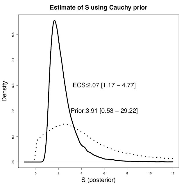
The median and 5-95% ranges for prior and posterior are also given. As you can see, the Cauchy prior doesn't really cut off the high tail that aggressively. In fact it's a lot higher than a U[0,10] or even U[0,20] prior would imply.
26 comments:
The difference between 1.1 - 4.4 and 1.2 - 4.8 doesn't seems worth worrying about too much especially as your Cauchy prior seems likely to exaggerate the upper tail?
.
Do you believe we can say that if S=10 or more, the paleo record would be highly likely to look different as in much more volatile as CO2 changed?
.
If S (equilibrium sensitivity to 2xCO2) was only 2 and CO2 has gone up by 41% or half a doubling, is it surprising that we have already warmed by one degree? Shouldn't there be more committed warming just waiting for the oceans to get up to temperature?
While this could easily be reconciled by warming caused by other than CO2, don't we largely know what effects these are and believe them to have an overall slight cooling effect?
I fail to understand why you do not start with a Levy distribution rather than the unphyiscal, in this case, Cauchy distribution.
David,
Levy? Just didn't think about it. I chose Cauchy as it was the fattest-tailed distribution that came to mind (borderline pathological). Was trying to avoid accusations that I'd just chosen a narrow prior to guarantee the result.
Chris,
Yes it's not so different with a Cauchy prior - perhaps not surprising as both have quadratic tails. However reverting to the old favourite uniform prior (which some people still argue for) does push up the 95% limit quite a bit, to 6.4 for 0-10 prior and over 8 for 0-20. So not hugely different from what has gone before, though the increased confidence in aerosol forcing is clearly cutting down the upper end gradually. Note that the 1C probably includes a bit of enso, it's not necessarily the true forced change. We'll have to wait and see how calculated estimates change in the next few years. Nic Lewis seems to still find ways of keeping the value down!
If you are going to call the Cauchy distribution you used pathological, doesn't this place a responsibility on you to come up with a believable prior?
Not sure if you can just take your Cauchy distribution and adjust it by cutting off all possibilities of S>25 or something crude like that or maybe something more sophisticated.
Anyway, showing the result with two different priors seems like a good idea. It should make it clearer that it is the data not the prior that is making the high sensitivities look unlikely, shouldn't it?
We'll have to wait and see how calculated estimates change in the next few years. Nic Lewis seems to still find ways of keeping the value down!
I think the key is stubborn refusal to accept that HadCRUT4 is biased low.
Based on CERES-EBAF data calibrated to Argo OHC up to July the 2008-2017 average TOA imbalance is going to be about 0.9W/m2, Berkeley Earth Land+Ocean global average about 1.01K difference from 1860-1879, forcing updated using NOAA AGGI to about 2.3W/m2.
Using base period imbalance of 0.08W/m2 following Otto et al. and 0.15W/m2 following Lewis and Curry, current median EffCS is then 2.5K and 2.4K respectively. (Making the prior mistakes you're talking about ;)
Even if surface temperatures and TOA imbalance stay at 2017 level for the next several years and don't increase further, EffCS will continue to trend upwards even with forcing increasing as normal.
Chris, let us not forget that our actual big problem is pushing carbon cycle feedbacks into unprecedentedly fast responses. That we can't really model them, and maybe of most concern the way they'll interact with each other, is unhelpful, especially since lots of modelers seem to want to pretend they don't exist. Did you know, BTW, that Earth System Sensitivity isn't, and that some paleos are worried about the prospect of a hyperthermal (driven mainly by tropical forest loss, not methane hydrates)?
>"that Earth System Sensitivity isn't"
isn't 'sensitive' doesn't seem to make sense. Isn't fixed perhaps?
Doesn't reflect the whole earth system. Permafrost loss and other potentially large carbon cycle feedbacks aren't included. If we're talking equilibrium conditions they don't need to be since they only operate during transients, but of course our near future isn't looking much like an equilibrium. This matters because the IPCC then ignores them, as do nearly all of the carbon budgets. Yes, the numbers are pretty speculative at this point, but assuming them to be zero is even more speculative.
>"Assuming them to be zero"
Most models take ghg levels as inputs. This is not taking carbon cycle feedbacks to be zero. When you do this, having 'decided'?? on a pathway, the available carbon budget is not (highest level - current level) but (highest level - current level - carbon feedbacks).
Those carbon feedbacks are currently negative rather than positive and it is not easy to spot much of a trend at present. I agree that a change in that trend will come but it isn't at all clear when or how quickly it will change.
This seems a good reason for erring on the side of caution, but doesn't seem a valid attack on climate scientists nor a reason to hype up short term equilibrium climate sensitivity which correctly avoids the issue by dealing with CO2 levels.
GHGs as inputs? As specified by the RCPs, which encompass a multitude of assumptions about the future but entirely elide key carbon cycle feedbacks. Please point to an IPCC model (GCM or ESM) that has incorporated the permafrost feedback described in Schuur et al. (2015).
OK, you can't model something if you can't describe the process and there's a good argument for not changing the RCPs, so maybe the carbon budgets are a better place to incorporate these feedbacks. But with one arguable exception, they don't.
This is fresh out of AGU FM, and illustrates the problem pretty well IMO.
[a rel="nofollow"]This[/a] is fresh ...
isn't very helpful
James,
Just out of interest is there a reasonable prior the completely excludes an ECS less than 1K and, if so, do you have a sense of what impact that would have on your posterior distribution?
No, I don't really think there are good arguments for excluding S less than 1 a priori and the data seem to rule that out fairly conclusively anyway so the answer is that I wouldn't want to do it but it wouldn't make any difference if I did!
James,
Thanks. Yes, the data does seem to largely rule that out. It seems to me that the prior is unlikely to significantly influence the range, but might impact the median, or what might be regarded as a best estimate. Do you think that is the case, or is the data strong enough that even the median is not particularly influenced by the choice of prior?
Oops. Let's try that link again.
ATTP,
No, since that whole region goes to zero (near enough) it won't make a difference. How the prior varies between 1 and 1.5 will matter, however.
Chris, this just popped up and seems highly pertinent, although they don't (can't) calculate the complete (i.e. including all slow feedbacks) sensitivity calculation. J + J have been asked to weigh in on this; hopefully one or the other or both will.
Also, re your comment above that it's "not easy to spot much of a trend at present," are you just going to ignore permafrost observations? Melillo et al. (2017) results are also relevant for the very near future. But if by "erring on the side of caution" you mean launching emergency action to reduce emissions, sure.
Thanks for the link.
"larger during interglacial states than during glacial conditions by more than a factor 2"
That seems worryingly small:
https://nas-sites.org/americasclimatechoices/files/2012/10/Figure-14.png
could suggest up to 15C change from CO2 change of 185 to 280 (.6 of a doubling) which could suggest a long term earth system climate sensitivity of 15/.6=25C.
I was hoping the glacial albedo effects would mean we could reduce above 25C by much more than a factor of 2. (Hence suggestion of 10C in first comment above for amount that perhaps could be ruled out.)
While no doubt above is terribly simplistic, am I getting calculations roughly right and what am I missing?
James' pathological cauchy prior might be sensible prior to such musings. After updating with such musings but before 20C data shouldn't a sensible prior diminish much more rapidly that quadratically after 25/2+a bit of a safety margin?
James,
How did you construct your Cauchy prior? It looks truncated at zero and I've looked at the Cauchy distro (I'm sort of guessing that you normalized a truncated Cauchy distro to unity).
What would happen if you repeatedly used the posterior as a 'so called' expert prior (e. g. update your prior with your posterior until it either collapses to a delta dirac like spike or has continuous drift or does it reach an asymptote (prior matches posterior).
Finally, what would happen if you truncated your prior at either +1 or +2 for the lower bound (i'm of the (perhaps naive) opinion that ECS isn't less than 2C and would like to see that as a firm lower bound foe any prior),
If I knew what I was doing ... which I don't ... I'd do this myself. Perhaps there is some prior art that you could point me to that gets a bit more radical than these IMHO rather flat priors (which also use a higher lower bound than zero).
Chris, I don't know where those numbers come from but the temperature is surely not global mean. Perhaps a local/polar estimate (and thus twice the global mean for starters). ESS of course assumes that the ice sheet amplifies CO2, maybe true in the colder past but we don't have much to lose now!
Everett, it's mostly described in this paper which is in climatic change a few years back. But in brief, it was intended to be a rather vague and long-tailed approximation to the opinions expressed in the Charney report. Repeatedly updating with the same data doesn't work, you just end up collapsing to a point. As I've said above I don't think the lower limit matters much and would be uncomfortable asserting that sensitivity cannot possibly be below 2C.
Thank you, yes of course it is local Antarctic temperature. (EPICA Dome C temperature anomaly based on original deuterium data interpolated to a 500-yr resolution) per https://www.nature.com/articles/nature06949
So such simple musing might make to put the peak of the prior after such musing but before 20C data at around 4-6 with only 50% chance of above that and tailing off fairly rapidly above say 12C? Or maybe there is much more to it like aerosol effects,.... ?
It seems you are not interested in suggesting a more reasonable prior if you are calling your Cauchy prior pathological.
So I doubt I will get anywhere with different approach. Still...
If your Cauchy prior is borderline pathologically wide, is it possible to suggest some other priors that look to you like:
borderline pathologically narrow
borderline pathologically high
borderline pathologically low
Is it then interesting to see what range of posterior PDFs you arrive at?
David Benson's suggestion of Levy might be good. But actually I think the prior is less of a issue nowadays, it's really more a question of how much faith we have in our understanding of the climate system and what the data actually mean...
Alternatively, avoid a prior by simply using the Bayes factor to determine which hypothesis best explains the data. This seems to have finally Caught On in molecular biology anyway. It ought to in climatology in my opinion.
Post a Comment