BlueSkiesResearch.org.uk: Like a phoenix redux

Even odder than finding that our old EnKF approach for parameter estimation was particularly well suited to the epidemiological problem, was finding that someone else had independently invented the same approach more recently…and had started using it for COVID-19 too!

In particular, this blogpost and the related paper, leads me to this 2013 paper wherein the authors develop a method for parameter estimation based on iterating the Kalman equations, which (as we had discovered back in in 2003) works much better than doing a single update step in many cases where the posterior is very small compared to the prior and the model is not quite perfectly linear – which is often the case in reality.

The basic idea behind it is the simple insight that if you have two observations of an unknown variable with independent Gaussian errors of magnitude e, this is formally equivalent to a single observation which takes the average value of the two obs, with an error of magnitude e/sqrt(2). This is easily shown by just multiplying the Gaussian likelihoods by hand. So conversely, you can split up a precise observation, with its associated narrow likelihood, into a pair of less precise observations, which have exactly the same joint likelihood but which can be assimilated sequentially in which case you use a broader likelihood, twice. In between the two assimilation steps you can integrate the model so as to bring the state back into balance with the parameters. It works better in practice because the smaller steps are more consistent with the linear assumptions that underpin the entire assimilation methodology.

This multiple data assimilation idea generalises to replacing one obs N(x_o,e) with n obs of the form N(x_o,e*sqrt(n)). And similarly for a whole vector of observations, with associated covariance matrix (typically just diagonal, but it doesn’t have to be). We can sequentially assimilate a lot of sets of imprecise obs in place of one precise set, and the true posterior is identical, but the multiple obs version often works better in practice due to generating smaller increments to the model/parameter samples and the ability to rebalance the model between each assimilation step.

Even back in 2003 we went one step further than this and realised that if you performed an ensemble inflation step between the assimilation steps, then by choosing the inflation and error scaling appropriately, you could create an algorithm that converged iteratively to the correct posterior and you could just keep going until it stopped wobbling about. This is particularly advantageous for small ensembles where a poor initial sample with bad covariances may give you no chance of reaching the true posterior under the simpler multiple data assimilation scheme.

I vaguely remembered seeing someone else had reinvented the same basic idea a few years ago and searching the deep recesses of my mind finds this paper here. It is a bit disappointing to not be cited by any of it, perhaps because we’d stopped using the method before they started….such is life. Also, the fields and applications were sufficiently different they might not have realised the methodological similarities. I suppose it’s such an obvious idea that it’s hardly surprising that others came up with it too.

Anyhow, back to this new paper. This figure below is a set of results they have generated for England (they preferred to use these data than accumulate for the whole of the UK, for reasons of consistency) where they assimilate different sets of data: first deaths, then deaths and hospitalised, and finally adding in case data on top (with some adjustments for consistency).

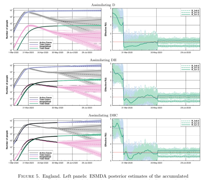
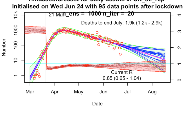
The results are broadly similar to mine, though their R trajectories seem very noisy with extremely high temporal variability – I think their prior may use independently sampled values on each day, which to my mind doesn’t seem right. I am treating R as taking a random walk with small daily increments except on lockdown day. In practice this means my fundamental parameters to be estimated are the increments themselves, with R on any particular day calculated as the cumulative sum of increments up to that time. I’ve include a few trajectories for R on my plot below to show what it looks like.

BlueSkiesResearch.org.uk: Like a phoenix…

So, the fortnightly chunks in the last post were doing ok, but it’s still a bit clunky. I quickly found that the MCMC method I was using couldn’t really cope with shorter intervals (meaning more R values to estimate). So, after a bit of humming and hawing, I dusted off the iterative Ensemble Kalman Filter method that we developed 15 years ago for parameter estimation in climate models I must put a copy up on our web site, it looks like there’s a free version here. For those who are interested in the method, the equations are basically the same as in the standard EnKF used in all sorts of data assimilation applications, but with a couple of tweaks to make it work for a parameter estimation scenario. It had a few notable successes back in the day, though people always sneered at the level of assumptions that it seemed to rely on (to be fair, I was also surprised myself at how well it worked, but found it hard to argue with the results).

And….rather to my surprise….it works brilliantly! I have a separate R value for each day, a sensible prior on this being Brownian motion (small independent random perturbation each day) apart from a large jump on lockdown day. I’ve got 150 parameters in total and everything is sufficiently close to Gaussian and linear that it worked at the first time of asking with no additional tweaks required. One minor detail in the application is that the likelihood calculation is slightly approximate as the algorithm requires this to be approximated by a (multivariate) Gaussian. No big deal really – I’m working in log space for the number of deaths, so the uncertainty is just a multiplicative factor. It means you can’t do the “proper” Poisson/negative binomial thing for death numbers if you care about that, but the reporting process is so much more noisy that I never cared about that anyway and even if I had, model error swamps that level of detail.

The main thing to tweak is how big a daily step to put into the Brownian motion. My first guess was 0.05 and that worked well enough. 0.2 is horrible, generating hugely noisy time series for R, and 0.01 is probably inadequate. I think 0.03 is probably about ok. It’s vulnerable to large policy changes of course but the changes we have seen so far don’t seem to have had much effect. I haven’t done lots of validation but a few experiments suggest it’s about right.

Here are a few examples where (top left) I managed to get a validation failure with a daily step of 0.01 (top right) used 0.2 per day but no explicit lockdown, just to see how it would cope (bottom left) same as top left but with a broader step of 0.03 per day (bottom right) the latest forecast.

I’m feeling a bit smug at how well it’s worked. I’m not sure what other parameter estimation method would work this well, this easily. I’ve had it working with an ensemble of 50, doing 10 iterations = 500 simulations in total though I’ve mostly been using an ensemble of 1000 for 20 iterations just because I can and it’s a bit smoother. That’s for 150 parameters as I mentioned above. The widely-used MCMC method could only do about a dozen parameters and convergence wasn’t perfect with chains of 10000 simulations. I’m sure some statisticians will be able to tell me how I should have been doing it much better…

Neoliberalism Kills?

However you "solve" the problem, the pandemic was always going to be very expensive. Government mandated lockdowns might be framed as the point at which the government disrupts market forces, decides to transfer some costs away from individuals, and to strongly shape the future trajectory.

The costs of lockdown vs no-lockdown in terms of both lives and money were probably not that well understood by the decision makers. While epidemiological models can easily predict 100s of thousands of deaths they assume no changes in behaviour by citizens. Rich countries with low inequality may reasonably hope for auto-lockdown by its citizens without such a massive interference by the government.  This has probably helped Japan, and perhaps to a lesser extent Sweden (Sweden has plenty of deaths but has also possibly kept more of its economy going..?). On the other hand, in many countries most people cannot afford to lockdown, and people not at such high risk (in this case, younger people) may feel much lower motivation to do so.

But instead of really thinking any of this through it seems that our dimwitted politicians simply applied their rubbish political ideological theories. They aren't scientists and do not know that theories have to make testable predictions in order to be worthwhile.

And what happened?! In this case socialism wins while neoliberalism both kills lots and lots of people and crashes the economy (because early lockdown => shorter lockdown). Ooops!

I would think it isn't always the case; socialist governments have surely fucked up very badly in the past when faced with other problems. That's the problem with random theories based on no evidence - they only work every so often. But I am still a bit worried that perhaps neoliberalism always kills and that this is just first chance to do a proper job of it.

The big caveat in all this is that we do not know what the endgame is. If herd immunity remains the inevitable consequence, then lockdown might be viewed in terms of the effect on quality of life in terms of months rather than in total lives saved. But those months are still pretty valuable, aren't they?

BlueSkiesResearch.org.uk: More COVID-19 parameter estimation

The 2 and now 3-segment piecewise constant approach seems to have worked fairly well but is a bit limited. I’m not really convinced that keeping R fixed for such long period and then allowing a sudden jump is really entirely justifiable, especially now we are talking about a more subtle and piecemeal relaxing of controls.

Ideally I’d like to use a continuous time series of R (eg one value per day), but that would be technically challenging with a naive approach involving a whole lot of parameters to fit. Approaches like epi-estim manage to generate an answer of sorts but that approach is based on a windowed local fit to case numbers, and I don’t trust the case data to be reliable. Also, this approach seems pretty bad when there is a sudden change as at lockdown, with the windowed estimation method generating a slow decline in R instead. Death numbers are hugely smoothed compared to infection numbers (due to the long and variable time from infection to death) so I don't think that approach is really viable.

So what I’m trying is a piecewise constant approach, with a chunk length to be determined. I’ll start here with 14 day chunks in which R is held constant, giving us say 12 R values for a 24 week period covering the epidemic (including a bit of a forecast). I choose the starting date to fit the lockdown date into the break between two chunks, giving 4 chunks before and 8 after in this instance.

I’ve got a few choices to make over the prior here, so I’ll show a few different results. The model fit looks ok in all cases so I’m not going to present all of them. This is what we get for the first experiment:

The R values however do depend quite a lot on the details and I’m presenting results from several slightly different approaches in the following 4 plots.

Top right left is the simplest version where each chunk has an independent identically distributed prior for R of N(2,1²). This is an example of the MCMC algorithm at the point of failure, in fact a little way past that point as the 12 parameters aren’t really very well identified by the data. The results are noisy and unreliable and it hasn’t converged very well. The last few values of R here should just sample the prior as there is no constraint at all on them. That they do such a poor job of that is an indication of what a dodgy sample it is. However it is notable that there is a huge drop in R at the right time when the lockdown is imposed, and the values before and after are roughly in the right ballpark. Not good enough, but enough to be worth pressing on with….

Next plot on top right is when I impose a smoothness constraint. R can still vary from block to block, but deviations between neighbouring values are penalised. The prior is still N(2,1²) for each value, so the last values of R trend up towards this range but don’t get there due to smoothness constraint. The result looks much more plausible to me and the MCMC algorithm is performing better too. However, the smoothness constraint shouldn’t apply across the lockdown as there was a large and deliberate change in policy and behaviour at that point.

So the bottom left plot has smoothness constraints applied before and after the lockdown but not across it. Note that the pre-lockdown values are more consistent now and the jump at lockdown date is even more pronounced.

Finally, I don’t really think a prior of N(2,1²) is suitable at all times. The last plot uses a prior of N(3,1²) before the lockdown and N(1,0.5²) after it. This is probably a reasonable representation of what I really think and the algorithm is working nicely.

Here is what it generates in terms of daily death numbers:

There is still a bit of of tweaking to be done but I think this is going to be a better approach than the simple 3-chunk version I’ve been using up to now.

Doubling times and the curious case of the dog that didn't bark

I'm sure many of you spend your mornings glued to Parliament TV but for anyone who missed it, there was a House of Lords Science and Technology Select Committee hearing on Tuesday, which discussed the science of Covid-19 with a particular focus on modelling. There are transcripts (two parts) here. and there is a video of the whole event here.

Two things particularly caught my attention. First bit is Question 31 in the transcript about 10:47ish when they are asked about the 20,000 death estimate that Vallance had hoped to undershoot. Matt Keeling first excused this by saying that the lockdown could have been stricter. However, Ferguson had already confirmed that the lockdown was in fact adhered to more strictly than the modellers had anticipated. (Keeling also went on to talk about the failure to protect care homes which is probably fair enough though the 20,000 target would have been badly overshot in any case). It would have surely been appropriate at this point to mention that the 20k target was already missed at the point that the lockdown was imposed on the 23rd March. By this point we had well over a million infected people, which already guaranteed well over 10k deaths, and there was no plausible way of stopping the outbreak dead in its tracks at that point. The decay was always going to be slower than the growth,  meaning more cases and deaths.

Then in the follow-up question, the witnesses were asked what had most surprised them compared to their earlier predictions. Ferguson answered with the biggest factor being that more infection had come from Spain and Italy and this is why they were further ahead on the curve than anticipated! The doubling time has nothing at all to do with how quickly people came with the infection, of course, and getting this wrong made a far greater difference to how things turned out.

It's curious that in two hours of discussion about the modelling, it never once came up that the modellers' estimate of the doubling time was 5-7 days up to the 18th march, and abruptly changed to 3-5 days on the 20th (reaching SAGE on the 23rd, according to the documentation)

The Dim and Dom show

I feel like I should be blogging about something related to the ongoing epidemic, but I can't bring myself to do it. The utterly vacuous, self-destructive, hopelessly incompetent nature of our government is beyond my ability to put into words. I am surprised at the scientists who are still prepared to work with them over the epidemic.

That aside, it's been an interesting couple of weeks. I'd been doing more of the same modelling and forecasting of the epidemic (and have updated our paper and submitted to a real journal), and then suddenly the media got hold of the delayed lockdown story. This is a very simple calculation, initially I thought too trivial to even write into a blog post, but it is of course very eye-catching. After mentions in the Guardian, Telegraph, More or Less, some requests for interviews came in. Initially I ducked them as I didn't really think it was appropriate for a non-expert to be pushing his own research especially as no-one else had backed it up at that point, and ATTP had tried to get results out of the IC model but initially came up with some significantly different answers (after a few more tries at getting the code to do the right things it worked very nicely though). Kit did a very good job on Sky I thought:

and then I found this manuscript (also written by an outsider, mathematical modeller like me) and the research showing essentially the same results for USA (manuscript here) (I think the smaller effect is mostly because they looked at a shorter interval) and also the Sunday Times article which managed to claim it was all new research from the IC team so I relented and did an interview for Vanessa Feltz on Radio 2 (which was live):



and also for the German channel ZDF which was recorded on Friday. Whether it will/did make the cut remains to be seen...the said they would send a link to the final version so I wait with bated breath.