BlueSkiesResearch.org.uk: EGU 2022 – how cold was the LGM (again)?

I haven’t blogged in ages but have actually done a bit of work. Specifically, I eventually wrote up my new reconstruction of the Last Glacial Maximum. We did this back in 2012/3 (see here) but since then there have been lots more model simulations, and then in 2020 Jessica Tierney published a new compilation and analysis of sea surface temperature proxy data. She also produced her own estimate of the LGM temperature anomaly based on this data set, coming up with -6.1±0.4C which seemed both very cold and very precise compared to our own previous estimate of -4.0±0.8C (both ranges at 95% probability).

We thought there were quite possibly some problems with her result, but weren’t a priori sure how important a factor this might have been, so that was an extra motivation to revisit our own work.

It took a while, mostly because I was trying to incrementally improve our previous method (multivariate pattern scaling) and it took a long time to get round to realising that what I really wanted was an Ensemble Kalman Filter, which is what Tierney et al (TEA) had already used. However, they used an ensemble made by sampling internal variability of a single model (CESM1-2) and a few different sets of boundary conditions (18ka and 21ka for LGM, 0 and 3ka for the pre-industrial), whereas I’m using the PMIP meta-ensemble of PMIP2, PMIP3, and PMIP4 models.

OK, being honest, that was part of the reason, the other part was general procrastination and laziness. Once I could see where it was going, tidying up the details for publication was a bit boring. But it got done, and the paper is currently in review at CPD. Our new headline result is -4.5±1.7C, so slightly colder and much more uncertain than our previous result, but nowhere near as cold as TEA.

I submitted an abstract for the EGU meeting which is on again right now. It’s fully blended in-person and on-line now, which is a fabulous step forwards that I’ve been agitating for from the sidelines for a while. They used to say it was impossible, but covid forced their hand somewhat with two years of virtual meetings, and now they have worked out how to blend it. A few teething niggles but it’s working pretty well, at least for us as virtual attendees. Talks are very short so rather than go over the whole reconstruction again (I’ve presented early versions previously) I focussed just on one question: why is our result so different from Tierney et al? While I hadn’t set out specifically to critique that work, the reviewers seemed keen to explore, so I’ve recently done a bit more digging into our result. My presentation can be found via this link, I think.

One might assume a major reason might be that the new TEA proxy data set was substantially colder than what went before, but we didn’t find that to be the case. In fact many of the gridded data points coincide physically with the MARGO SST data set which we had previously used, and the average value over these locations was only 0.3C colder in TEA than MARGO (though there was a substantial RMS difference between the points, which is interesting in itself as it suggests that these temperature estimates may still be rather uncertain). A modest cooling of 0.3 in the mean for these SST points might be expected to translate to about 0.5 or so for surface air temperature globally, not close to to the 2.1C difference seen between our 2013 result and their 2020 paper. Also, our results are very similar when we switch between using MARGO and TEA and both together. So, we don’t believe the new TEA data are substantially different from what went before.

What is really different between TEA and our new work is the priors we used.

Here is a figure summarising our main analysis, which follows the Ensemble Kalman Filter approach, which means we have a prior ensemble of model simulations (lower blue dots, summarised in the blue gaussian curve above) each of which is updated by nudging towards observations, generating the posterior ensemble of upper red dots and red curve. I’ve highlighted one model in green, which is CESM1-2. Under this plot I have pasted bits of a figure from Tierney et al which shows their prior and posterior 95% ranges. I lined up the scales carefully. You can see that the middle of their ensembles, which are entirely based on CESM1-2, are really quite close to what we get with the CESM1-2 model (the big dots in their ranges are the median of their distributions, which obviously aren’t quite gaussian). Their calculation isn’t identical to what we get with CESM1-2, because it’s a different model simulation, with different forcing, we are using different data and there are various other differences in the details of our calculation. But it’s close.

Here is a terrible animated gif. It isn’t that fuzzy in the full presentation. What it shows is the latitudinal temperatures (anomalies relative to pre-industrial) of our posterior ensemble of reconstructions (thin black lines, thick line showing the mean), with the CESM-derived member highlighted in green, and Tierney et al’s mean estimate added in purple. The structural similarity between those two lines is striking.

A simple calculation also shows that the global temperature field of our CESM-derived sample is closer to their mean in the RMS difference sense, than any other of our ensemble members. Clearly, there’s a strong imprint of the underlying model even after the nudge towards the data sets.

So, this is why we think their result is largely down to their choice of prior. While we have a solution that looks like their mean estimate, this lies close to the edge of our range. The reason they don’t have any solutions that look like the bulk of our results is simply that they excluded them a priori. It’s nothing to do with their new data or their analysis method.

We’ve been warning against the use of single model ensembles to represent uncertainty in climate change for a full decade now, it’s disappointing that the message doesn’t seem to have got through.

BlueSkiesResearch.org.uk: How to do emergent constraints properly

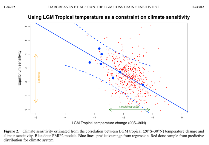
Way back in the mists of time, we did a little bit of work on "emergent constraints". This is a slightly hackneyed term referring to the use of a correlation across an ensemble of models between something we can’t measure but want to estimate (like the equilibrium climate sensitivity S) and something that we can measure like, say, the temperature change T that took place at the Last Glacial Maximum….

Actually our early work on this sort of stuff dates back 15 years but it was a bit more recently, in 2012 when we published this result

in the paper blogged about here that we started to think about it a little more carefully. It is easy to plot S against T and do a linear regression, but what does it really mean and how should the uncertainties be handled? Should we regress S on T or T on S? [I hate the arcane terminology of linear regression, the point is whether S is used to predict T (with some uncertainty) or T is used to predict S (with a different uncertainty)]. We settled for the conventional approach in the above picture, but it wasn’t entirely clear that this was best.

And is this regression-based approach better or worse than, or even much the same as, using a more conventional and well-established Bayesian Model Averaging/Weighting approach anyway? We raised these questions in the 2012 paper and I’d always intended to think about it more carefully but the opportunity never really arose until our trip to Stockholm where we met a very bright PhD student who was interested in paleoclimate stuff and shortly afterwards attended this workshop (jules helped to organise this: I don’t think I ever got round to blogging it for some reason). With the new PMIP4/CMIP6 model simulations being performed, it seemed a good time to revisit any past-future relationships and this prompted us to reconsider the underlying theory which has until now remained largely absent from the literature.

So, what is new our big idea? Well, we approached it from the principles of Bayesian updating. If you want to generate an estimate of S that is informed by the (paleoclimate) observation of T, which we write as p(S|T), then we use Bayes Theorem to say that

p(S|T) ∝ p(T|S)p(S).

Note that when using this paradigm, the way for the observations T to enter in to the calculation is via the likelihood p(T|S) which is a function that takes S as an input, and predicts the resulting T (probabilistically). Therefore, if you want to use some emergent constraint quasi-linear relationship between T and S as the basis for the estimation then it only really makes sense to use S as the predictor and T as the predictand. This is the opposite way round to how emergent constraints have generally (always?) been implemented in practice, including in our previous work.

So, in order to proceed, we need to create a likelihood p(T|S) out of our ensemble of climate models (ie, (T,S) pairs). Bayesian linear regression (BLR) is the obvious answer here – like ordinary linear regression, except with priors over the coefficients. I must admit I didn’t actually know this was a standard thing that people did until I’d convinced myself that this must be what we had to do, but there is even a wikipedia page about it.

This therefore is the main novelty of our research: presenting a way of embedding these empirical quasi-linear relationships described as "emergent constraints" in a standard Bayesian framework, with the associated implication that it should be done the other way round.

Given the framework, it’s pretty much plain sailing from there. We have to choose priors on the regression coefficients – this is a strength rather than a weakness in my view, as it forces us to explicitly consider whether we consider the relationship to be physically sound, and argue for its form. Of course it’s easy to test the sensitivity of results to these prior assumptions. The BLR is easy enough to do numerically, even without using the analytical results that can be generated for particular forms of priors. And here’s one of the results in the paper. Note that unlabelled x-axis is sensitivity in both of these plots, in contrast to being the y-axis in the one above.

While we were doing this work, it turns out that others had also been thinking about the underlying foundations of emergent constraints, and two other highly relevant papers were published very recently. Bowman et al introduces a new framework which seems to be equivalent to a Kalman Filter. In the limit of a large ensemble with a Gaussian distribution, I think this is also equivalent to a Bayesian weighting scheme. One aspect of this that I don’t particularly like is the implication that the model distribution is used as the prior. Other than that, I think it’s a neat idea that probably improves on the Bayesian weighting (eg that we did in the 2012 paper) in the typical case that we have where the ensemble is small and sparse. Fitting a Gaussian is likely to be more robust than using a weighted sum of a small number of samples. But, it does mean you start off from the assumption that the model ensemble spread is a good estimator for S, which is therefore considered unlikely to like outside this range. Whereas regression allows us to extrapolate, in the case where the observation is at our outside the ensemble range.

The other paper by Williamson and Sansom presented a BLR approach which is in many ways rather similar to ours (more statistically sophisticated in several aspects). However, they fitted this machinery around the conventional regression direction. This means that their underlying prior was defined on the observation with S just being an implied consequence. This works ok if you only want to use reference priors (uniform on both T and S) but I’m not sure how it would work if you already had a prior estimate of S and wanted to update that. Our paper in fact shows directly the effect of using both LGM and Pliocene simulations to sequentially update the sensitivity.

The limited number of new PMIP4/CMIP6 simulations means that our results are substantially based on older models, and the results aren’t particularly exciting at this stage. There’s a chance of adding one or two more dots on the plots as the simulations are completed, perhaps during the review process depending how rapidly it proceeds. With climate scientists scrambling to meet the IPCC submission deadline of 31 Dec, there is now a huge glut of papers needing reviewers…

More word salad

Having accused someone else of writing a word salad it's only fair that I should tar jules with the same brush too :-) Life as an unemployed self-employed scientist isn't all holidays and bison burgers, she occasionally does some work too though coincidentally (or not) her latest paper is the result of another trip to the USA a couple of years ago. Unfortunately someone didn't get the open access memo hence my link is to the sci-hub copy. Writs to /dev/null please.

It's a review and thus should be accessible to a wide audience, but monsoon dynamics is a fair way outside my comfort zone so I don't really have much to say about it. The abstract appears to have a rather low Flesch Reading Ease score of 6.8: for comparison my first paragraph above rates 51 (the scores are out of 100, with higher numbers more readable) so I think I've got a good excuse. I think the main conclusion is that more research is needed, and that if someone could come up with a better all-encompassing theory that explained it all, that would be really great. From the paleo perspective (which is where jules comes in) there is the well-known Problem of the Green Sahara, being that there was significant (vegetation-supporting) precipitation in this region during the mid-Holocene, which models cannot adequately explain or represent.

Here's a diagram about monsoon dynamics:

Well, that's about it from me. Still on holiday but we've got some work lined up and will be be returning to it in the near future.

BlueSkiesResearch.org.uk: Ich bin ein Hamburger

We are currently at MPI Hamburg courtesy of Thorsten Mauritsen. Just here for the week but planning a longer visit later in the year. I haven’t been here before, and jules has not particularly great memories of a brief meeting elsewhere in Hamburg 20 years ago, so the city has been a pleasant surprise so far. Got here yesterday just in time for a jog to the lake and back in the Sunday afternoon sun, followed by a somewhat disappointing hamburger,  so hopefully we’ll have a chance to put that right later this week.

First thing this morning we gave short seminars which was great timing as it now means everyone else knows who we are and what we’ve been doing. That’s something we failed to manage so well at NCAR last year. Most of the joint interest concerns the use of paleoclimate simulations to test and validate different versions of their new/forthcoming climate model.

The building is interesting though jules can’t help but wonder if disillusioned modellers are ever tempted to take the short-cut down from the 4th floor…

BlueSkiesResearch.org.uk: Blueskies tour of the USA

The possibility of visiting NCAR has been at the back of our minds for some time, so when the rare honour of invitations to speak at the AGU Fall Meeting in San Francisco plopped into both of our inboxes around June, we swung into action. A couple of months at NCAR rounded off with an easy hop to SF seemed too good an opportunity to miss, so jules sent an email to Bette who leads the paleo group at NCAR to ask if she could host us. There was a bona-fide research reason for the visit, in that we are hoping to extend/supersede this work (and simultaneously improve on this reconstruction!) by blending together model simulations with proxy data records to create a complete reanalysis of the last deglaciation, 21ka to the present. There’s a forthcoming PMIP-supported plan for GCMs to simulate this entire period (the main instigators being next door in Leeds is a happy coincidence), but this may take a couple of years to actually happen, as 21 thousand years of simulation is a huge task for complex models. However, Bette is ahead of the pack having done this a few years ago with a slightly lower resolution model, so our plan was to use her model output (among other things) to work out how to do it in the meantime. The view from (near) NCAR Having started to arrange the visit, we then started fishing around for support and found out that NCAR (subsistence) and PEN (travel including AGU costs) were prepared to help us pay for the trip, for which we were and are very grateful. Then to top it off, another invitation arrived, for a workshop on "model dependence and sampling strategies in climate model ensemble prediction"…to be held at NCAR in early December, immediately prior to the AGU! I expect that the organiser Gab Abramowitz was really only inviting me out of politeness with no expectation that I’d fly there for a two day meeting at my own expense (they had no money for this) but of course we were now planning to be there so I was delighted to be able to accept. It then turned out that Reto Knutti was already at NCAR on a year’s sabbatical, and a couple of his ex/current students who were working in this area and are now also supervised by Gab visited briefly en route to the AGU along with Gab. We arrived in mid-October, though our luggage did not. Our departure from Leeds had been a bit disorganised, as the computer system there was down and all check-in/luggage drop had to be by done by hand. The resulting delay gave us a tighter than planned connection at Heathrow (including a terminal change) and therefore it wasn’t a great surprise that our checked baggage with hand-written tags didn’t turn up in Denver. So our first couple of days in Boulder were filled with emergency shopping (along with scrounging some free googlewear off our friend Rob who works there). Fortunately all our stuff turned up over the following week, albeit in 3 separate deliveries all in the middle of the night which did nothing for the jet lag. Most of the luggage consisted of two travelling bicycles (S&S couplers) which we had used some 19 years previously on my first visit to Boulder. That didn’t end so well – for us or the bikes (evidence) – when we met a Harley-Davidson on the wrong side of one of the twisty canyon roads, but fortunately there were no similar incidents this time around. Boulder is great for cycling around, being pretty much flat with a sunny dry climate and a wonderful network of bike/pedestrian paths many of which follow various creeks though and across town. Boulder creek and its path Our apartment was an easy distance for cycling (and sometimes running) to work, 6km direct (though with a 250m climb) with a range of longer options for more energetic days. NCAR also runs their own regular shuttle up to the lab and there’s good public transport in Boulder, so we didn’t plan to hire a car for our stay though thought we might do so for one or two weekend trips to the surrounding countryside and national parks. In fact in the end we forgot to pack our driving licenses so couldn’t do this, which didn’t turn out to be much of a hardship as there was enough to keep us busy in the vicinity of the town. Just outside the town, there are some huge hills to climb and some decent mountain biking. The indirect way to work… …and the really long way home! NCAR is really well set up for visiting, there were several offices set aside for the use of visitors and we were up and running with ID cards and computers and internet access etc in a couple of hours on our first day, which would not likely have happened at JAMSTEC, or anywhere else we’ve been before. There’s also a very good canteen which we made the most of, even including some breakfasts. NCAR seems to be on everyone’s itinerary – there were many seminars from short-term visitors, and it was quite a surprise to bump into someone we knew from Bristol who was also passing through. So just being there was a good opportunity to meet with a range of people, though in fact our main work on the deglaciation turned out to be largely self-contained. Snow usually appears around the middle of October in Boulder, but we were lucky to arrive during a particularly dry autumn and had a full month of warm sunny weather during which we made full use of Boulder’s various leisure opportunities. We quickly bought some cheap old MTB tyres from Community Cycles and enjoyed visits to Dowdy Draw, the West Magnolia Drive trail area, and Marshall Mesa. Somewhere on the trails We also climbed up most of the mountain roads – Magnolia Drive to Nederland, Flagstaff, through Jamestown to Rob’s place and finally up and down Lee Hill Drive. West Magnolia trails I also found a few of the local running groups and went out for a couple of rather gentle Sunday morning runs with the Boulder Roadrunners and more challenging runs with the Boulder Track Club who seemed to consist of quick to super-fast runners. Luckily the runs were basically out and back routes so I could watch them all zoom off into the distance and after turning round a bit early they would all zoom past me on the way back too. jules and I together joined the Trailrunners for the first hour of one of their monster mountain marathon days. We just went up Flagstaff but most of the rest went all the way to Bear Peak and back, about 24 miles with a lot of climbing. The work went well, though it’s far from finished and so we don’t have a lot to report yet. We  presented this poster at the AGU which summarised our research so far: In short, it looks like at a minimum the basic idea should succeed fine but it’s a bit early to say anything about what the overall result will look like, and there are plenty of opportunities for improving on the very simple method we used. It will also be very helpful to get some more PMIP simulations but we may have to wait some time for these, so there’s no great rush for the methodology but we will keep working on it as time allows. Towards the end of our visit, just about when we were starting to get a bit bored with sitting in an office and working on the deglaciation, we had to shift gears to prepare not only for the AGU meeting but also for the workshop on climate model ensembles. In all we had 4 presentations to give on entirely unrelated topics in a bare week (me talking twice, jules once, and a joint poster). I don’t think anything from the workshop is available on the web (it was a rather small and informal affair) but there are plans to write some sort of review paper. There was no real breakthrough but there was hopefully some shared understanding of the different ideas that people have come up with. I’ve also got a month to revise this manuscript, and now have a significant improvement to put in to it. Although the new idea didn’t arise directly at the meeting, having to give a presentation about it and field questions afterwards did provoke the inspiration. By this time the snow had arrived, giving a very different feel to the daily commute. We didn’t really have enough winter clothing and temperatures down to -20C (with a daily max of -10C) were a bit of a struggle, though it looked pretty when not actually snowing: A snowy ride Straight after the workshop we flew over to San Francisco for the AGU meeting, about which I’ll write separately. For now you can make do with the view from our hotel window (on the one sunny morning we had). We came back and had a couple of days in Boulder, just enough to empty our office and tidy up the apartment and pack all our stuff for the long haul back to the UK. No drama on that trip, and a bizarre lack of jet lag following our return, perhaps because it’s so peaceful and dark at night here in Settle that there’s really no excuse to stay awake. While we were in the USA, it seemed like there was some sort of election going on. The result didn’t go down well with most (perhaps all!) of the staff at NCAR. I hope the institute survives for other people to have as enjoyable and useful visits as we did!