BlueSkiesResearch.org.uk: Science breakthrough of the year (runner-up)

Being only a small and insignificant organisation, we would like to take this rare opportunity to blow our own trumpets.

Blue Skies Research contributed to one of the runners-up in Science Magazine’s “Breakthrough of the year” review! Specifically, the estimation of climate sensitivity that I previously blogged about here.

Obviously, were it not for the pesky virus, we would have won outright.

BlueSkiesResearch.org.uk: Back to the future

Way back in the mists of time (ie, 2006), jules and I saw what was going on with people estimating climate sensitivity, and in particular how this literature was interpreted by the authors of the IPCC AR4. And we didn’t like it. We thought that any reasonable synthesis should consider the multiple lines of evidence in a coherent fashion in order to form a credible overall view. This resulted in the paper "Using multiple observationally‐based constraints to estimate climate sensitivity" described in this blog post (paper here), which people unfamiliar with the story might like to glance at before progressing further…

It’s fair to say that our intervention was not met by universal approval at the time, with the established researchers mostly finding excuses as to why our result might not be entirely trustworthy. Fine, do your own calculations, we said. And they didn’t.

Time passed, and a new generation of people with different backgrounds became interested in estimating climate sensitivity. The World Climate Research Program (WCRP) made it a central theme in one of their Grand Challenges in climate science. There were a couple of meetings in Ringberg that jules and then I attended sequentially.

In 2016, several of leaders of this WCRP steering group wrote a paper which kicked off a project to perform a new synthesis of the evidence on climate sensitivity. Their idea was to form an overall synthesis of the multiple lines of evidence, roughly along the lines that we had originally proposed, but in a far more comprehensive and thorough fashion. This is something that the IPCC isn’t really equipped to do, as it just assesses and summarises the literature. The project leaders considered three main strands of evidence: that arising from process studies (ie the behaviour of clouds, including simulations from GCMs), the transient warming over the historical record, and paleoclimate. Jules was one of the lead authors for the paleo chapter, but I wasn’t involved at the outset. However when invited to join the group I was of course happy to contribute to it, having thought about the problem off and on for the past decade.

Writing it was a lengthy and at times frustrating process, due to the huge range of ideas, topics, backgrounds and knowledge of the author team. That is also what gives this review its strength, of course, as we have genuine experts in multiple areas of modelling and data analysis, covering a huge range of time scales and techniques, and the different perspectives meant we gave each other quite a workout in testing the robustness of our approaches and ideas. During the 4 year process we had regular videoconferences, typically 9pm UK time, being 6am for Japan, 10am in Australia and afternoon for the continental USA. Luckily we had an 8-9h gap in the global spread so no-one actually had to get up in the middle of the night each time! We also had a single major writing meeting in Edinburgh in summer 2018 which almost all the main authors were able to attend in person, and a handful of "meet-ups of opportunity" when subsets happened to go to other conferences. In all, it was good practice for the new normal that we are enjoying due to COVID.

The peer review was probably the most extensive I’ve experienced, with something like 10 sets of comments – this was something we were all keen on, as we suspected it would be beyond the compass of just the usual 2-3 people. Comments were basically encouraging but gave us quite a lot to work on and in fact we reorganised the paper substantially for the better resulting in the 2nd set of reviews being very positive. Finally got it done a couple of months ago and it was accepted subject to very minor corrections (which were mostly things we had spotted ourselves, in fact).

The new paper has now been published, actually I’m not entirely sure it is up yet (minor snafu on the embargo timing) but anyone who needs an urgent look can find it here. I may write more on the details if pressed, but for now here is a quick peek at the main results:

The "baseline" calculation is what we get from putting together all the evidence, with a resulting 2.6-3.9C "likely" range. The coloured curves are various sensitivity tests, with the purple line at the top defined as the range from the lowest 17th percentile, and the highest 83rd percentile, across these tests. This isn’t really a probability range and doesn’t correspond to any particular calculation.

BlueSkiesResearch.org.uk: Bayesian deconstruction of climate sensitivity estimates using simple models: implicit priors and the confusion of the inverse

Has just been published!

It wasn’t really my intention, but somehow we never came up with a proper title so now we’re stuck with it!

This paper was born out of our long visit to Hamburg a few years ago, from some discussions relating to estimates of climate sensitivity. It was observed that there were two distinct ways of analysing the temperature trend over the 20th century: you could either (a): take an estimate of forced temperature change, and an estimate of the net forcing (accounting for ocean heat uptake) and divide one by the other, like Gregory et al, or else (b): use an explicitly Bayesian method in which you start with a prior over sensitivity (and an estimate of the forcing change), perform an energy balance calculation and update according to how well the calculation agrees with the observed warming, like this paper (though that one uses a slightly more complex model and obs – in principle the same model and obs could have been used though).

These give slightly different answers, raising the question of (a) why? and (b) is there a way of doing the first one that makes it look like a Bayesian calculation?

This is closely related to an issue that Nic Lewis once discussed many years ago with reference to the IPCC AR4, but that never got written up AFAIK and is a bit lost in the weeds. If you look carefully, you can see a clue in the caption to Figure 1, Box 10.1 in the AR4 where it says of the studies:

some are shown for different prior distributions than in the original studies

Anyway, there is a broader story to tell, because this issue also pops up in other areas including our own paleoclimate research (slaps wrist). The basic point we try to argue in the manuscript is that when a temperature (change) is observed, it can usually be assumed to be the result of a measurement equation like:

T_O = T_T + e        (1)

where T_O is the numerical value observed, T_T is the actual true value, and e is an observational error which we assume to be drawn from a known distribution, probably Gaussian N(0,σ²) though it doesn’t have to be. The critical point is that this equation automatically describes a likelihood P(T_O|T_T) and not a probability distribution P(T_T|T_O), and we claim that when researchers interpret a temperature estimate directly as a probability distribution in that second way they are probably committing a simple error known as “confusion of the inverse” which is incredibly common and often not hugely important but which can and should be avoided when trying to do proper probabilistic calculations.

Going back to equation (1), you may think it can be rewritten as

T_T = T_O  + e       (2)

(since -e and e have the same distribution) but this is not the same thing at all because all these terms are random variables and e is actually independent of T_T, not T_O.

Further, we show that in committing the confusion of the inverse fallacy, researchers can be viewed as implicitly assuming a particular prior for the sensitivity, which probably isn’t the prior they would have chosen had they thought about it more explicitly.

The manuscript had a surprisingly (to me) challenging time in review, with one reviewer in particular taking exception to it. I encourage you to read their review(s) if you are interested. We struggled to understand their comments initially, but think their main point was that when a researcher writes down a pdf for T_T such as N(T_O,σ²) it was a bit presumptuous of us to claim they had made an elementary error in logical reasoning when they might in fact have been making a carefully considered Bayesian estimate taking account of all their uncertainties.

While I think in theory it’s possible that they could be right in some cases, I am confident that in practice they are wrong in the vast majority of cases including all the situations under consideration in our manuscript. For starters, if their scenario was indeed the case, the question would not have arisen in the first place as all the researchers working on these problems would already have understood fully what they did and why. And one of the other cases in the manuscript was based on our own previous work, where I’m pretty confident in remembering correctly that we did this wrong But readers can make up their own minds as to how generally applicable it is. It’s an idea, not a law.

Our overall recommendation is that people should always try to take the approach of the Bayesian calculation, as this makes all their assumptions explicit. It would have been a bit embarrassing if it had been rejected, because a large and wildly exciting manuscript which makes extensive use of this idea has just been (re-)submitted somewhere else today.  Watch this space!

I think this is also notable as the first time we’ve actually paid paper charges in the past few years – on previous occasions we have sometimes pleaded poverty, but now we’ve had a couple of contracts that no long really applies. Should get it free really as a reward for all the editing work – especially by jules!

BlueSkiesResearch.org.uk:What can we learn about climate sensitivity from interannual variability?

Another new manuscript of ours out for review, this time on ESDD. The topic is as the title suggests. This work grew out of our trips to Hamburg and later Stockholm though it wasn’t really the original purpose of our collaboration. However, we were already working with a simple climate model and the 20th century temperature record when the Cox et al paper appeared (previous blogs here, here, here) so it seemed like an interesting and relevant diversion. Though the Cox et al paper was concerned with emergent constraints, this new manuscript doesn’t really have any connection to this one I blogged earlier though it is partly for the reasons explained in that post that I have presented the plots with S on the x-axis.

A fundamental point about emergent constraints, which I believe is basically agreed upon by everyone, is that it’s not enough to demonstrate a correlation between something you can measure and something you want to predict, you have to also present a reasonable argument why you expect this relationship to exist. With 10^6 variables to choose from in your GCM output (and an unlimited range of functions/combinations thereof) it is inevitable that correlations will exist, even in totally random data. So we can only reasonably claim that a relationship has predictive value if it has a theoretical foundation.

The use of variability (we are taking about the year-to-year variation in global mean temperature here after any trend has been removed) to predict sensitivity has a rather chequered history. Steve Schwartz tried and failed to do this, perhaps the clearest demonstration of this failure being that the relationship he postulated to exist for the climate system (founded on a very simple energy balance argument) did not work for the climate models. Cox et al sidestepped this pitfall by the simple and direct technique of presenting a relationship which had been directly derived from the ensemble of CMIP models, so by construction it worked for these. They also gave a reasonable-looking theoretical backing for the relationship, which was based on an analysis of a very simple energy balance argument. So on the face of it, it looked reasonable enough. Plenty of people had their doubts though as I’ve documented in the links above.

Rather than explore the emergent constraint aspect in more detail, we chose to approach the problem from a more fundamental perspective: what can we actually hope to learn from variability? We used the paradigm of idealised “perfect model” experiments, which enables us to generate very clear limits to our learning. The model we used is more-or-less the standard two layer energy balance of Winton, Held etc that has been widely adopted, but with a random noise term (after Hasselmann) added to the upper layer to simulate internal variability:

The single layer model that Cox et al used in their theoretical analysis is also recovered when the ocean mixing parameter γ is set to zero. So now the basic question we are addressing is, how accurately can we diagnose the sensitivity of this energy balance model, from analysis of the variability of its output? 

Firstly, we can explore the relationship (in this model) between sensitivity S and the function of variability which Cox et al called ψ.

Focussing firstly on the fat grey dots, these represent the expected value of ψ from an unforced (ie, due entirely to internal variability) simulation of the single-layer energy balance model that Cox et al used as the theoretical foundation for their analysis. And just as they claimed, these points lie on a straight line. So far so good.

But…

It is well known that the single layer model does a pretty shabby job at representing GCM behaviour during the transient warming over the 20th century, and the two-layer version of the energy balance model gives vastly superior results for only a small increase in complexity. (This is partly why the Schwartz approach failed). Repeating our analysis with the two-layer version of the model, we get the black dots, where the relationship is clearly nonlinear. This model was in fact considered by the Cox group in a follow-up paper Williamson et al in which they argued that it still displayed a near-linear relationship between S and ψ over the range of interest spanned by GCMs. That’s true enough as the red line overlying the plot shows (I fitted that by hand to the 4 points in the 2-5C range) but there’s also a clear divergence from this relationship for larger values of S.

And moreover…

The vertical lines through each dot are error bars. These are the ±2 standard deviation ranges of the values of ψ that were obtained from a large sample of simulations, each simulation being 150 years long (a generous estimate of the observational time series we have available to deal with). It is very noticeable that the error bars grow substantially with S. This together with the curvature in the S-ψ relationship means that it is quite easy for a model with a very high sensitivity to generate a time series that has a moderate ψ value. The obvious consequence being that if you see a time series with a moderate ψ value, you can’t be sure the model that generated it did not have a high sensitivity.

We can use calculations of this type to generate the likelihood function p(ψ|S), which can be thought of as a horizontal slice though the above graph at a fixed value of ψ, and turn the handle of the Bayesian engine to generate posterior pdfs for sensitivity, based on having observed a given value of ψ. This is what the next plot shows, where the different colours of the solid lines refer to calculations which assumed observed values for ψ of 0.05, 0.1, 0.15 and 0.2 respectively.

These values correspond to the expected value of ψ you get with a sensitivity of around 1, 2.5, 5 and 10C respectively. So you can see from the cyan line that if you observe a value of 0.1 for ψ, that corresponds to a best estimate sensitivity of 2.5C in this experiment, you still can’t be very confident that the  true value wasn’t rather a lot higher. It is only when you get a really small value of ψ that the sensitivity is tightly constrained (to be close to 1 in the case ψ=0.05 shown by the solid dark blue line).

The 4 solid lines correspond to the case where only S is uncertain and all other model parameters are precisely known. In the more realistic case where other model parameters such as ocean heat uptake are also somewhat uncertain, the solid blue line turns into the dotted line and in this case even the low sensitivity case has significant uncertainty on the high side.

It is also very noticeable that these posterior pdfs are strongly skewed, with a longer right hand tail than left hand (apart from the artificial truncation at 10C). This could be directly predicted from the first plot where the large increase in uncertainty and flattening of the S-ψ relationship means that ψ has much less discriminatory power at high values of S. Incidentally, the prior used for S in all these experiments was uniform, which means that the likelihood is the same shape as the plotted curves and thus we can see that the likelihood is itself skewed, meaning that this is an intrinsic property of the underlying model, rather than an artefact of some funny Bayesian sleight-of-hand. The ordinary least squares approach of a standard emergent constraint analysis doesn’t acknowledge or account for this skew correctly and instead can only generate a symmetric bell curve.

One thing that had been nagging away at me was the fact that we actually have a full time series of annual temperatures to play with, and there might be a better way of analysing them than to just calculate the ψ statistic. So we also did some calculations which used the exact likelihood of the full time series p({Ti}|S) where {Ti}, i = 1…n is the entire time series of temperature anomalies. I think this is a modest novelty of our paper, no-one else that I know of has done this calculation before, at least not quite in this experimental setting. The experiments below assume that we have perfect observations with no uncertainty, over a period of 150 years with no external forcing. Each simulation with the model generates a different sequence of internal variability, so we plotted the results from 20 replicates of each sensitivity value tested. The colours are as before, representing S = 1, 2.5 and 5C respectively. These results give an exact answer to the question of what it is possible to learn from the full time series of annual temperatures in the case of no external forcing.

So depending on the true value of S, you could occasionally get a reasonably tight constraint, if you are lucky, but unless S is rather low, this isn’t likely. These calculations again ignore all other uncertainties apart from S and assume we have a perfect model, which some might think just a touch on the optimistic side…

So much for internal variability. We don’t have a period of time in the historical record in which there was no external forcing anyway, so maybe that was a bit academic. In fact some of the comments on the Cox paper argued (and Cox et al acknowledged in their reply) that the forced response might be affecting their calculation of ψ, so we also considered transient simulations of the 20th century and implemented the windowed detrending method that they had (originally) argued removed the majority of the forced response. The S-ψ relationship in that case becomes:

where this time the grey and black dots and bars relate not to one and two layer models, but whether S alone is uncertain, or whether other parameters beside S are also considered uncertain. The crosses are results from a bunch of CMIP5 models that I had lying around, not precisely the same set that Cox et al used but significantly overlapping with them. Rather than just using one simulation per model, this plot includes all the ensemble members I had, roughly 90 model runs in total from about 25 models. There appears to be a vague compatibility between the GCM results and the simple energy balance model, but the GCMs don’t show the same flattening off or wide spread at high sensitivity values. Incidentally the set of GCM results plotted here don’t fit a straight line anywhere nearly as closely as the set Cox et al used. It’s not at all obvious to me why this is the case, and I suspect they just got lucky with the particular set of models they had combined with the specific choices they made in their analysis.

So it’s no surprise that we get very similar results when looking at detrended variability arising from the forced 20th century simulations. I won’t bore you with more pictures as this post is already rather long. The same general principles apply.

The conclusion is that the theory that Cox et al used to justify their emergent constraint analysis, actually refutes their use of a linear fit using ordinary least squares, because the relationship between S and ψ is significantly nonlinear and heteroscedastic (meaning the uncertainties are not constant but vary strongly with S). The upshot is that any constraint generated from ψ – or even more generally, any constraint derived from internal or forced variability – is necessarily going to be skewed with a tail to high values of S. However, variability does still have the potential to be somewhat informative about S and shouldn’t be ignored completely, which many analyses based on the long-term trend automatically do.

BlueSkiesResearch.org.uk: How to do emergent constraints properly

Way back in the mists of time, we did a little bit of work on "emergent constraints". This is a slightly hackneyed term referring to the use of a correlation across an ensemble of models between something we can’t measure but want to estimate (like the equilibrium climate sensitivity S) and something that we can measure like, say, the temperature change T that took place at the Last Glacial Maximum….

Actually our early work on this sort of stuff dates back 15 years but it was a bit more recently, in 2012 when we published this result

in the paper blogged about here that we started to think about it a little more carefully. It is easy to plot S against T and do a linear regression, but what does it really mean and how should the uncertainties be handled? Should we regress S on T or T on S? [I hate the arcane terminology of linear regression, the point is whether S is used to predict T (with some uncertainty) or T is used to predict S (with a different uncertainty)]. We settled for the conventional approach in the above picture, but it wasn’t entirely clear that this was best.

And is this regression-based approach better or worse than, or even much the same as, using a more conventional and well-established Bayesian Model Averaging/Weighting approach anyway? We raised these questions in the 2012 paper and I’d always intended to think about it more carefully but the opportunity never really arose until our trip to Stockholm where we met a very bright PhD student who was interested in paleoclimate stuff and shortly afterwards attended this workshop (jules helped to organise this: I don’t think I ever got round to blogging it for some reason). With the new PMIP4/CMIP6 model simulations being performed, it seemed a good time to revisit any past-future relationships and this prompted us to reconsider the underlying theory which has until now remained largely absent from the literature.

So, what is new our big idea? Well, we approached it from the principles of Bayesian updating. If you want to generate an estimate of S that is informed by the (paleoclimate) observation of T, which we write as p(S|T), then we use Bayes Theorem to say that

p(S|T) ∝ p(T|S)p(S).

Note that when using this paradigm, the way for the observations T to enter in to the calculation is via the likelihood p(T|S) which is a function that takes S as an input, and predicts the resulting T (probabilistically). Therefore, if you want to use some emergent constraint quasi-linear relationship between T and S as the basis for the estimation then it only really makes sense to use S as the predictor and T as the predictand. This is the opposite way round to how emergent constraints have generally (always?) been implemented in practice, including in our previous work.

So, in order to proceed, we need to create a likelihood p(T|S) out of our ensemble of climate models (ie, (T,S) pairs). Bayesian linear regression (BLR) is the obvious answer here – like ordinary linear regression, except with priors over the coefficients. I must admit I didn’t actually know this was a standard thing that people did until I’d convinced myself that this must be what we had to do, but there is even a wikipedia page about it.

This therefore is the main novelty of our research: presenting a way of embedding these empirical quasi-linear relationships described as "emergent constraints" in a standard Bayesian framework, with the associated implication that it should be done the other way round.

Given the framework, it’s pretty much plain sailing from there. We have to choose priors on the regression coefficients – this is a strength rather than a weakness in my view, as it forces us to explicitly consider whether we consider the relationship to be physically sound, and argue for its form. Of course it’s easy to test the sensitivity of results to these prior assumptions. The BLR is easy enough to do numerically, even without using the analytical results that can be generated for particular forms of priors. And here’s one of the results in the paper. Note that unlabelled x-axis is sensitivity in both of these plots, in contrast to being the y-axis in the one above.

While we were doing this work, it turns out that others had also been thinking about the underlying foundations of emergent constraints, and two other highly relevant papers were published very recently. Bowman et al introduces a new framework which seems to be equivalent to a Kalman Filter. In the limit of a large ensemble with a Gaussian distribution, I think this is also equivalent to a Bayesian weighting scheme. One aspect of this that I don’t particularly like is the implication that the model distribution is used as the prior. Other than that, I think it’s a neat idea that probably improves on the Bayesian weighting (eg that we did in the 2012 paper) in the typical case that we have where the ensemble is small and sparse. Fitting a Gaussian is likely to be more robust than using a weighted sum of a small number of samples. But, it does mean you start off from the assumption that the model ensemble spread is a good estimator for S, which is therefore considered unlikely to like outside this range. Whereas regression allows us to extrapolate, in the case where the observation is at our outside the ensemble range.

The other paper by Williamson and Sansom presented a BLR approach which is in many ways rather similar to ours (more statistically sophisticated in several aspects). However, they fitted this machinery around the conventional regression direction. This means that their underlying prior was defined on the observation with S just being an implied consequence. This works ok if you only want to use reference priors (uniform on both T and S) but I’m not sure how it would work if you already had a prior estimate of S and wanted to update that. Our paper in fact shows directly the effect of using both LGM and Pliocene simulations to sequentially update the sensitivity.

The limited number of new PMIP4/CMIP6 simulations means that our results are substantially based on older models, and the results aren’t particularly exciting at this stage. There’s a chance of adding one or two more dots on the plots as the simulations are completed, perhaps during the review process depending how rapidly it proceeds. With climate scientists scrambling to meet the IPCC submission deadline of 31 Dec, there is now a huge glut of papers needing reviewers…

BlueSkiesResearch.org.uk: Marty Weitzman: Dismally Wrong.

De mortuis nil nisi bonum and all that, but I realise I only wrote this down in a very abbreviated and perhaps unclear form many years ago, in fact prior to publication of the paper it concerns. I was sad to hear of his untimely death and especially by suicide when he surely had much to offer. But like all innovative researchers, he made mistakes too, and his Dismal Theorem was surely one of them. Since it’s been repeatedly brought up again recently, I thought I should explain why it’s wrong, or perhaps to be more precise, why it isn’t applicable or relevant to climate science in the way he presented it.

His basic claim in this famous paper was that a “fat tail” (which can be rigorously defined) on a pdf of climate sensitivity is inevitable, and leads to the possibility of catastrophic outcomes dominating any rational economic analysis. The error in his reasoning is, I believe, rather simple once you’ve seen it, but the number of people sufficiently well-versed in statistics, climate science and economics (and sufficiently well-motivated to carefully examine the basis of his claim) is approximately zero so as far as I’m aware no-one else ever spotted the problem, or at least I haven’t seen it mentioned elsewhere.

The basic paradigm that underpins his analysis is that if we try to estimate the parameters of a distribution by taking random draws from it, then our estimate of the distribution is going to naturally take the form of a t-distribution which is fat-tailed. And importantly, this remains true even when we know the distribution to be Gaussian (thin-tailed), but we don’t know the width and can only estimate it from the data. The presentation of this paradigm is hidden beyond several pages of verbiage and economics which you have to read through first, but it’s clear enough on page 7 onwards (starting with “The point of departure here”).

The simple point that I have to make is to observe that this paradigm is not relevant to how we generate estimates of the equilibrium climate sensitivity. We are not trying to estimate parameters of “the distribution of climate sensitivity”, in fact to even talk of such a thing would be to commit a category error. Climate sensitivity is an unknown parameter, it does not have a distribution. Furthermore, we do not generate an uncertainty estimate by comparing a handful of different observationally-based point estimates and building a distribution around them. (Amusingly, if we were to do this, we would actually end up with a much lower uncertainty than usually stated at the 1-sigma level, though in this case it could indeed end up being fat-tailed in the Weitzman sense.) Instead, we have independent uncertainty estimates attached to each observational analysis, which are based on analysis of how the observations are made and processed in each specific case. There is no fundamental reason why these uncertainty estimates should necessarily be either  fat- or thin-tailed, they just are what they are and in many cases the uncertainties we attach to them are a matter of judgment rather than detailed mathematical analysis. It is easy to create artificial toy scenarios (where we can control all structural errors and other “black swans”) where the correct posterior pdf arising from the analysis can be of either form.

Hence, or otherwise, things are not necessarily quite as dismal as they may have seemed.

BlueSkiesResearch.org.uk: Steffen nonsense

Been pondering whether it was worth bother blogging this but I haven’t written for a while and in the end I decided the title was too good a pun to pass on (I never claimed to have high standards).

The paper "Trajectories of the Earth System in the Anthropocene" had entirely passed me by when it came out, though it did seem to attract a bit of press coverage eg with the BBC saying

Researchers believe we could soon cross a threshold leading to boiling hot temperatures and towering seas in the centuries to come.
Even if countries succeed in meeting their CO2 targets, we could still lurch on to this “irreversible pathway”.
Their study shows it could happen if global temperatures rise by 2C.
An international team of climate researchers, writing in the journal, Proceedings of the National Academy of Sciences, says the warming expected in the next few decades could turn some of the Earth’s natural forces – that currently protect us – into our enemies.

and continues in a similar vein quoting an author

“What we are saying is that when we reach 2 degrees of warming, we may be at a point where we hand over the control mechanism to Planet Earth herself,” co-author Prof Johan Rockström, from the Stockholm Resilience Centre, told BBC News.
“We are the ones in control right now, but once we go past 2 degrees, we see that the Earth system tips over from being a friend to a foe. We totally hand over our fate to an Earth system that starts rolling out of equilibrium.”

Like I said, I had missed this, and it was only an odd set of circumstances that led me to read it, about which more below. But first, the paper itself. The illustrious set of authors postulate that once the global temperatures reach about 2C above pre-industrial, a set of positive feedbacks will kick in such that the temperature will continue to rise to about 5C above pre-industrial, even without any further emissions and direct human-induced warming. Ie, once we are going past +2C, we won’t be able to stabilise at any intermediate temperature below +5C.

The paper itself is open access at PNAS. The abstract is slightly more circumspect, claiming only that they "explore the risk":

We explore the risk that self-reinforcing feedbacks could push the Earth System toward a planetary threshold that, if crossed, could prevent stabilization of the climate at intermediate temperature rises and cause continued warming on a "Hothouse Earth" pathway even as human emissions are reduced. Crossing the threshold would lead to a much higher global average temperature than any interglacial in the past 1.2 million years and to sea levels significantly higher than at any time in the Holocene.

(the paper fleshes out these words in numerical terms).

The paper lists a number of possible positive carbon cycle feedbacks and quantifies them as summing to a little under half a degree of additional warming (Table 1 in the paper). The authors then wave their hands, say it could all get much worse, and with one bound Jack was free. End of paper. I went through it again to see what I’d missed, and I really hadn’t. It is just make-believe, they don’t "explore the risk" at all, they just assert it is significant. There’s a couple of nice schematic graphics about tipping points too.

The mildly interesting part is what led me to read the paper at all, 6 months after missing its original publication. An editor contacted me a little while ago to ask if I’d write half a of debate (to form a book chapter) over whether exceeding 2C of warming would lock us onto a trajectory for a much warmer hothouse earth. I was charged with arguing the sceptical side of that claim. I was initially a bit baffled by the proposal as I had not (at that point) thought anyone had claimed anything to the contrary, but it soon became clear what it was all about. I said I’d be happy to oblige, but it turns out that my intended opponents, being two of the co-authors on the paper itself, were not prepared to defend it in those terms.

BlueSkiesResearch.org.uk: Comments on Cox et al

And to think a few weeks ago I was thinking that not much had been happening in climate science…now here’s another interesting issue. I previously blogged quite a lot about the Cox et al paper (see here, here, here). It generated a lot of interest  in the scientific community and I’m not terribly surprised that it provoked some comments which have just been published and which can be found here (along with the reply) thanks to sci-hub.

My previous conclusion was that I was sceptical about the result, but that the authors didn’t seem to have done anything badly wrong (contrary to the usual situation when people generate surprising results concerning climate sensitivity). Rather, it seemed to me like a case of a somewhat lucky result when a succession of reasonable choices in the analysis had turned up an interesting result. It must be noted that this sort of fishing expedition does invalidate any tests of statistical significance and thus also invalidates the confidence intervals on the Cox et al result, but I didn’t really want to pick on that  because everyone does it and I thought that hardly anyone would understand my point anyway

The comments generally focus on the use of detrended intervals from the 20th century simulations. This was indeed the first thing that came to my mind as a likely Achilles’ heel of the Cox et al analysis. I don’t think I showed it previously, but the first thing I did when investigating their result was to have a play with the ensemble of simulations that had been performed with the MPI model. The Cox et al analysis depends on an estimate of the lag-1 autocorrelation of the annual temperatures of the climate models. Ideally, if you want to calculate the true lag-1 autocorrelation of model output, you should use a long control run (ie an artificial simulation in which there is no external forcing). Of course there is no direct observational constraint on this, but nevertheless this is one of the model parameters involved in the Cox et al constraint, for which they claim a physical basis.

As well as having a long control simulation of the MPI model, there is also a 100-member of 20th century simulations using it. The size of this ensemble means that as well as allowing an evaluation of the Cox et al detrending approach to estimate the autocorrelation,  we can also test another approach which is to remove the ensemble average (which represents the forced response) rather than detrending a single simulation.

This figure shows the results I obtained. And rather to my surprise….there is basically no difference. At least, not one worth worrying about. For each of the three approaches, I’ve plotted a small sample from the range of empirical results (the thin pale lines) with the thicker darker colours showing the ensemble mean (which should be a close approximation to the true answer in each case). For the control run I used short chunks comparable in length to the section of 20th century simulation that Cox et al used. The only number that actually matters from this graph is the lag-1 value which is around 0.5, the larger lags are just shown for fun. The weak positive values from 5-10 years probably represent the influence of the model’s El Nino. It’s clear that the methodological differences here are small both in absolute terms and also relative to the sample variation across ensemble members. That is to say, sections of control runs, or 20th century simulations which are either detrended or which have the full forced response removed, all have a lag-1 autocorrelation of about 0.5 albeit with significant variation from sample to sample.

Of course this is only one model out of many, and may not be repeated across the CMIP ensemble, but this analysis suggested to me that this detrending approach wasn’t a particularly important issue and so I did not pursue it further. It is interesting to see how heavily the comments focus on it. It seems that the authors of these got different results when they looked at the CMIP ensemble.

One thing I’d like to mention again, which the comments do not, is that the interannual variability of the CMIP models is actually more strongly related to sensitivity, than either the autocorrelation or Cox’s Psi function (which involves both these parameters) are. Here is a the plot I showed earlier. Which is of course a little bit dependent on the outlying data points (as was commented on my original post). This is sensitivity vs SD (calculated from the control runs) of the CMIP models of course.

I don’t know why this is so, I don’t know whether it’s important, and I’m surprised that no-one else bothered to mention it as interannual variability is probably rather less sensitive than autocorrelation is to the detrending choices. Maybe I should have written a comment myself

In their reply to the comments. Cox et al now argue that their use of a simple detrending means that their analysis includes a useful influence of some of the 20th century forced response, which "sharpens" the relationship with sensitivity (which is weaker when the CMIP control runs are used). This seems a bit weak to me and as well as basically contradicting their original hypothesis, also breaks one of the fundamental principles of emergent constraints, that they should have a clear physical foundation. At the end of the discussion I’m more convinced that the windowing and detrending is a case of "researcher degrees of freedom" ie post-hoc choices that render the statistical analysis formally invalid. It’s an interesting hypothesis rather than a result.

The real test will be applying the Cox et al analysis to the CMIP6 models, although even in this case intergenerational similarity makes this a weaker challenge  than would be ideal. I wonder if we have any bets as to what the results will be?

BlueSkiesResearch.org.uk: That new ocean heat content estimate

From Resplandy et al (conveniently already up on sci-hub):

Our result — which relies on high-precision O2 measurements dating back to 1991 — suggests that ocean warming is at the high end of previous estimates, with implications for policy- relevant measurements of the Earth response to climate change, such as climate sensitivity to greenhouse gases

But how big are these implications? As it happens I was just playing around with 20th century energy balance estimates of the climate sensitivity, so I could easily plug in the new number. My calc is based on a number of rough estimates so is not intended to be definitive but should show the general effect fairly realistically.

I was previously using the Johnson et al 2016 estimate of ocean heat uptake which is 0.68W/m^2 (on a global mean basis). Resplandy et al raise this value to 0.83. Their paper presents their value as a rather more substantial increase by comparing to an older value that the IPCC apparently gave.

Plugging the numbers in to a standard energy balance approximation we get the following estimates for the equilibrium sensitivity:

This simple calculation has a (now) well-known flaw that tends to bias the results low, though how low is up for debate (it’s the so-called "pattern effect" or you might know it as the difference between effective and equilibrium sensitivity). I used my preferred Cauchy prior from this old paper. It has a location parameter of 2.5 and a scale factor of 3 (meaning it should have a median of 2.5 and interquartile range of -0.5 – 5.5, though it’s truncated here at 0 and 10 for convenience). 

The old calculation based on Johnson et al’s ocean heat uptake has a median of  2.35C with a 5-95% range of 1.41 – 4.61C. The new estimate raises this to a median of 2.57C with a range of 1.53 – 5.17C. So, about 0.1C on the bottom end and 0.5C on the top end, which may not be the impression the manuscript gives. The medians and ranges are shown with the tick marks. The calculation goes up to 10C but I truncated the plot at 6C (and thus cut off the prior’s 95% limit) for clarity.

Another caveat in my calculation is that the new paper’s main result is based on a longer time interval going back to 1991, if the ocean heat uptake has been accelerating then that would imply a larger increment to the Johnson et al figure (which relates to a more recent period) and thus a larger effect. But even so it’s an incremental change, and not earth-shattering. As one might expect for such a well-studied phenomenon.

BlueSkiesResearch.org.uk: Cox et al part 3

As promised some more on this. The first thing I thought, on seeing this paper – a feeling that others apparently shared – was, why had no-one else already thought of this? Had we all just behaved like the fabled economist who, when their companion points out a £10 note lying on the pavement, ignores it, saying "If there really was a £10 note, someone would have picked it up already"?

Certainly the Schwartz fiasco will have put people off from pursuing this approach, as many of us had shown via a variety of arguments that the theoretical relationship in the simple 1-box climate model that directly links the autocorrelation of internal variability to equilibrium response, cannot be directly used for diagnosing the latter from the former in more complex climate models. Of course, this is not quite what Cox et al do, rather they show a strong correlation between their measure of variability and the sensitivity, across the ensemble of CMIP5 models. One complication in their analysis is that they measure variability via the 20th century simulations. Most of the variation in temperature seen in the 20th century is actually the response to external forcing and this forcing is far from the white noise assumed by Cox et al’s analysis (even after detrending, the variation about the trend is not white noise either). This would seem to undermine the theoretical basis for their relationship.

So, rather than using the 20th century simulations, I’ve had a quick look at the pre-industrial control simulations in which models are run for lengthy periods of time with no changes in external forcing. In all the following analyses I have restricted my attention to the models for which I had at least 500y of P-I control simulation, in order that the behaviour of each model would be well characterised (it is well known that the empirical estimate of the lag-1 autocorrelation tends to be biased low to a substantial degree for short time series). This restricted my set to 13 models. In this set of 13 models I  included both the MIROC models (5 and ESM) which Cox et al used as alternates, as I happen to know that the changes between the two generations here are substantial and were specifically made to affect the climate sensitivity-relevant processes as can be seen in their widely differing equilibrium sensitivities. It may however be that my results are themselves somewhat sensitive to the choice of models.

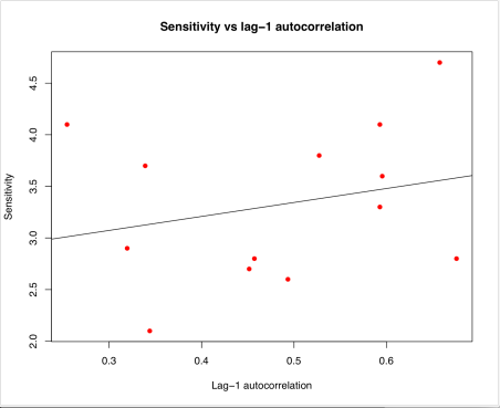
So, firstly, here’s a quick look at whether the lag-1 autocorrelation of annual mean temperature is related to the equilibrium sensitivity across this set of models:

Nope. The regression line is nearly flat and nowhere near significant.

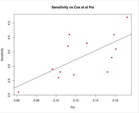
However, this isn’t quite what Cox et al presented. They actually calculated a function psi which depends also on the magnitude of interannual variability as well as its persistence. In fact their psi is defined as sd/sqrt(-log(alpha)) were sd is the standard deviation of interannual variability and alpha is the lag-1 correlation coefficient. They argue that this is the most relevant diagnostic as it is linearly related to sensitivity in their theoretical case. Sure enough when we calculate psi for the control simulations and correlate this with sensitivity we see:

There is a significant correlation at the 5% level! Just to be clear, the values of psi here are not the same ones that Cox et al calculate, instead I’ve applied their formula to the model data from the control simulations in order to eliminate the effect of external forcing. So why does this work whereas the lag-1 autocorrelation is not useful?

Well the answer is found by checking the relationship between standard deviation (the numerator in their psi function) and sensitivity, and here it is:

This is actually a much stronger correlation than the previous one, now significant at the 1% level. Of course we have no direct measure of the magnitude of internal variability of the real climate system, but this could be reasonably estimated by subtracting the forced response from the observations (by some combination of statistical and/or model-based calculation). So this relationship could in principle also be used as an emergent constraint (without prejudice as to its credibility).

In terms of the simple one-box climate model, the differing magnitudes of interannual variability across the ensemble could be due to the variation in (internally-generated) radiative imbalance on the interannual time scale, or the effective heat capacity of the thin layer that reacts on this time scale, or the radiative feedback lambda = 1/sensitivity. I suppose more detailed examination of model data might reveal which factor is most important here. I would be very surprised if people haven’t already looked into this in some detail, and don’t propose to do so myself at this point. Certainly many people have looked at variability on various space and time scales and tried to relate this to equilibrium sensitivity. Anyway, at this point I think I should call a halt and "reach out to" (don’t you hate that phrase) Andy Dessler and perhaps one or two others to ask if this strong correlation makes sense to them. I can’t help but think it would have been noticed previously if it’s actually robust (eg if it exists across CMIP3 as well as CMIP5). And if not, maybe it’s just luck.

BlueSkiesResearch.org.uk: More about Cox et al.

Time to move this discussion onto the BlueSkiesResearch blog as it is, after all, directly related to my work. Previous post here but I might copy that over here too.

Conversations about the Cox et al paper have continued on twitter and blogs. Firstly, Rasmus Benestad posted an article on RealClimate that I thought missed the mark rather badly. His main complaint seems to be that the simple model discussed by Cox et al doesn’t adequately describe the behaviour of the climate system over short and long time scales. Of course that’s well known but Cox et al explicitly acknowledge this and don’t actually use the simple model to directly diagnose the climate sensitivity. Rather, they use it as motivation for searching for a relationship between variability and sensitivity, and for diagnosing what functional form this relationship might take. Since a major criticism of the emergent constraint approach is that it risks data mining and p-hacking to generate relationships out of random noise, it’s clearly a good thing to have some theoretical basis for them, as jules and I have frequently mentioned in the context of our own paleoclimate research.

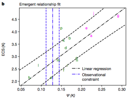
And more recently, Tapio Schneider has posted an article arguing that Cox et al underestimated their uncertainties. Unfortunately, he does this via an analysis of his own work that certainly does underestimate uncertainties, but which does not (I believe) accurately represent the Cox et al work. Here’s the Cox et al figure again, and below it another regression analysis of different data from Schneider’s blog.

It’s clear at a glance that the uncertainty bounds on the Cox et al regression basically include most of the models whereas the uncertainty bounds of Schneider exclude the vast majority of his (I’m talking about the black dashed lines in both plots). I think the simple error here is that Schneider is considering only the uncertainty on the regression line itself whereas Cox is considering the predictive uncertainty of the regression relationship. The theoretical basis for most of the emergent constraint work is that reality can be considered to be "like" one of the models in the sense of satisfying the regression relationship that the models exhibit, ie it follows on naturally from the statistically indistinguishable paradigm for ensemble interpretation (I don’t preclude the possibility that there may be other ways to justify it). The intuitive idea is that reality is just like another model for which we can observe the variable on the x-axis (albeit typically with some non-negligible uncertainty) and want to predict the corresponding variable on the y-axis. So the location of reality along the x-axis is constrained by our observations of the climate system, and it is likely to be a similar distance from the regression line as the models themselves are.

Schneider then compares his interpretation of the emergent constraint method with model weighting, this being a fairly standard Bayesian approach. We also did this in our LGM paper, though we did the regression method properly so the differences were less marked. I always meant to go back and explore the ideas underlying the two approaches in more detail, but I believe that the main practical difference is that the Bayesian weighting approach is using the models themselves as a prior whereas the regression is implicitly using a uniform prior on the unknown. The regression has the ability to extrapolate beyond the model range and also can be used more readily when there is a very small number of models, as is typically the case in paleo research.

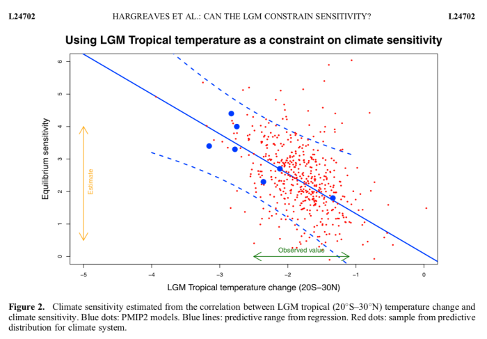
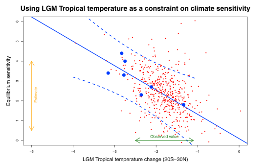
Here’s our own example from the paper which attempts to use tropical temperature at the Last Glacial Maximum as a constraint on the equilibrium sensitivity.

The models are the big blue dots (yes, only 7 of them, hence the large uncertainty in the regression). I used the random sampling (red dots) to generate the pdf for sensitivity, by first sampling from the pdf for tropical temperature and then for each dot sampling from the regression prediction. The broad scatter of the red dots is due to using t-distributions which I think is necessary due to the small number of models involved (eg even the uncertainty on the tropical temp constraint is a t-distribution as it was estimated by a leave-one-out cross validation process). But this is perhaps a bit of a fine detail on the overall picture. It is often not clear exactly how other authors have approached this and to be fair it probably matters less when considering modern constraints when data are generally more precise and ensemble sizes are rather larger.

We also did the Bayesian model weighting in this paper, but with only 7 models the result is a bit unsatisfactory. However the main reason we didn’t like it for that work is that by using the models as a prior, it already constrains the sensitivity substantially! Whereas if the observations of LGM cooling had been outside the model range, the regression would have been able to extrapolate as necessary.

Here’s the weighting approach applied to the same question, with the blue dots marking the models, the green curve is the prior pdf (equal weighting on the models) and the thick red is the posterior which is the weighted sum of the thinner red curves. Each model has to be dressed up in a rather fat gaussian kernel (standard techniques exist to choose an appropriate width) to make an acceptably smooth shape. It’s different from the regression-based answer, but not radically so, and the difference can for the most part be attributed to the different prior.

Having said all that, I’m not uncritically a fan of the Cox et al work and result, a point that I’ll address in a subsequent post. But I thought I should point out that at least these two criticisms of Schneider and Benestad seem basically unfounded and unfair.