We refer the interested reader to Betteridge’s Law. End of post.
Ok, I will add a little more. This is the title of our latest (last?) paper, which came out a couple of months ago. The work was a long time in progress, despite being in principle a fairly run-of-the-mill application of our previously-developed methods to a new time period. While the work was underway, we got hold of a new data set (and new collaborators) which meant doing it all over again, though that’s not sufficient to explain my overall slowness. Anyway it’s done now.
The mid-Pliocene Warm Period (which could perhaps more precisely be referred to as the mid-Piacenzian Warm Period, we had some discussion with reviewers about this but argued it wasn’t our responsibility to enforce the less-widely-used name on the community, especially as we were using outputs from the Pliocene Modelling Intercomparison Projects) is the most recent period when the climate was thought to be substantially warmer than the pre-industrial state, for a significant period of time. But it was more than 3 million years ago, so data are sparse and imprecise, and boundary conditions (such as atmospheric CO2 level) are also not that well known. Nevertheless, lots of modelling groups have performed simulations of this period, and others have collected proxy data pertaining to the same time.
We basically repeated our recent(ish) work on the Last Glacial Maximum, using the model simulations and proxy data…..and as part of this, compared results obtained with different types of proxy data. Unfortunately these disagreed substantially, which led us to conclude that we really can’t provide a very confident answer. And even if we assume that one data set is correct, we still have significant uncertainty over the result generated. Our (weakly) preferred number is 3.6 +- 1C warmer than pre-industrial, but I wouldn’t claim to be too confident about that. That’s pretty much it, really. “More work is necessary” is actually true in this instance.
We did produce a bunch of pictures, such as this one, which shows the central estimate of surface air temperature anomaly across the globe. But the regional detail of the patterns isn’t reliable (such as the occasional spots of cooling). It’s just…that’s what the algorithm churned out.
Way back in the mists of time (ie, 2006), jules and I saw what was going on with people estimating climate sensitivity, and in particular how this literature was interpreted by the authors of the IPCC AR4. And we didn’t like it. We thought that any reasonable synthesis should consider the multiple lines of evidence in a coherent fashion in order to form a credible overall view. This resulted in the paper "Using multiple observationally‐based constraints to estimate climate sensitivity" described in this blog post (paper here), which people unfamiliar with the story might like to glance at before progressing further…
It’s fair to say that our intervention was not met by universal approval at the time, with the established researchers mostly finding excuses as to why our result might not be entirely trustworthy. Fine, do your own calculations, we said. And they didn’t.
Time passed, and a new generation of people with different backgrounds became interested in estimating climate sensitivity. The World Climate Research Program (WCRP) made it a central theme in one of their Grand Challenges in climate science. There were a couple of meetings in Ringberg that jules and then I attended sequentially.
In 2016, several of leaders of this WCRP steering group wrote a paper which kicked off a project to perform a new synthesis of the evidence on climate sensitivity. Their idea was to form an overall synthesis of the multiple lines of evidence, roughly along the lines that we had originally proposed, but in a far more comprehensive and thorough fashion. This is something that the IPCC isn’t really equipped to do, as it just assesses and summarises the literature. The project leaders considered three main strands of evidence: that arising from process studies (ie the behaviour of clouds, including simulations from GCMs), the transient warming over the historical record, and paleoclimate. Jules was one of the lead authors for the paleo chapter, but I wasn’t involved at the outset. However when invited to join the group I was of course happy to contribute to it, having thought about the problem off and on for the past decade.
Writing it was a lengthy and at times frustrating process, due to the huge range of ideas, topics, backgrounds and knowledge of the author team. That is also what gives this review its strength, of course, as we have genuine experts in multiple areas of modelling and data analysis, covering a huge range of time scales and techniques, and the different perspectives meant we gave each other quite a workout in testing the robustness of our approaches and ideas. During the 4 year process we had regular videoconferences, typically 9pm UK time, being 6am for Japan, 10am in Australia and afternoon for the continental USA. Luckily we had an 8-9h gap in the global spread so no-one actually had to get up in the middle of the night each time! We also had a single major writing meeting in Edinburgh in summer 2018 which almost all the main authors were able to attend in person, and a handful of "meet-ups of opportunity" when subsets happened to go to other conferences. In all, it was good practice for the new normal that we are enjoying due to COVID.
The peer review was probably the most extensive I’ve experienced, with something like 10 sets of comments – this was something we were all keen on, as we suspected it would be beyond the compass of just the usual 2-3 people. Comments were basically encouraging but gave us quite a lot to work on and in fact we reorganised the paper substantially for the better resulting in the 2nd set of reviews being very positive. Finally got it done a couple of months ago and it was accepted subject to very minor corrections (which were mostly things we had spotted ourselves, in fact).
The new paper has now been published, actually I’m not entirely sure it is up yet (minor snafu on the embargo timing) but anyone who needs an urgent look can find it here. I may write more on the details if pressed, but for now here is a quick peek at the main results:
The "baseline" calculation is what we get from putting together all the evidence, with a resulting 2.6-3.9C "likely" range. The coloured curves are various sensitivity tests, with the purple line at the top defined as the range from the lowest 17th percentile, and the highest 83rd percentile, across these tests. This isn’t really a probability range and doesn’t correspond to any particular calculation.
We were supposed to be in Vienna, but that was all cancelled a while back of course. I might have felt sorry for my AirBnB host but despite Austria banning everything they didn’t reply to my communication and refused a refund so when AirBnB eventually (after a lot of ducking and weaving) stepped in and over-ruled them and gave me my money back I didn’t have much sympathy. They weren’t our usual host, who was already full when I booked a bit late this year.
Rather than the easy option of just cancelling the meeting, the EGU decided to put everything on-line. They didn’t arrange videoconferencing sessions – I think this was probably partly due to the short notice, and also to make everything as simple and accessible as possible to people who might not have had great home broadband or the ability to use streaming software – but instead we had on-line chat (typing) sessions with presentation material previously uploaded by authors, that we could refer to as we liked. There was no formal division into posters and oral presentations. Authors could put up whatever they wanted (50MB max) onto the website beforehand and people were free to download and browse through at will. It is all still up there and available to all permanently, and you can comment on individual presentations up to the end of the month (assuming the authors have allowed this, which most seem to). The EGU has posted this blog with statistics of attendance which shows it to have been an impressive success.
Some people put up huge presentations, far more than they would have managed in a 15 minute slot, but most were more reasonable and presented a short summary. We did poster format for ours as we felt that this allowed more space for text explanation and an easier browsing experience than a sequence of slides with bullet points. Unfortunately my personal program of sessions I had decided to attend has been deleted from the system so I can’t review what I saw in much detail. I usually take notes but this time was too busy with computer screens.
Of course, being in Vienna in spirit, I had to have a schnitzel. I might have to have some more in the future, they were rather good and quite easy to make. Pork fillet, not veal.
The 2nd portion at the end of the week was better as I made my own breadcrumbs rather than using up some ancient panko that was skulking in the back of the cupboard. But we ate them too quickly to take pictures! Figlmüller eat your heart out!
The chat sessions were a bit frenetic. Mostly, the convenors invited each author in turn to post a few sentences in summary, following which there was a short Q-and-A free-for all. This only allowed for about 5 mins per presentation, which meant maybe 2 or 3 questions. But this wasn’t quite as bad as it seems since it was easy to scroll through the uploaded material ahead of time and pick out the interesting ones. Questioning could also run over subsequent presentations, it wasn’t too hard to keep track of who was asking what if you made the effort. As usual, there were only handful of interesting presentations per session for me (at most) so it was easy enough to focus on these. It was also possible to be in several different chat sessions at once, which you can’t do so easily with physical presentations! The structure made it more feasible to focus on whatever piqued our interest, and jules in particular spent more time at those sessions she does not usually get around to attending because they are outside of her main focus. Some convenors grouped presentations into themes and discussed 3-5 of them at a time, for longer. Some naughty convenors thought they would be clever and organise videoconferencing sessions outside of the EGU system, which actually worked pretty well in practice for those (probably a large majority to be honest) who could access it, but not so good for those who had access blocked for a number of reasons. Which is probably why the EGU didn’t organise this themselves. Whether it is actually preferable to the on-line chat is a matter of taste.
Jules was co-convening a couple of sessions and the convenors set up a small zoom session on the side to help coordinate, which added to the fun. A bit of personal chat with colleagues is an important aspect of these conferences. Her presentation is here and outlines some early steps in some work we are currently doing – an update to our previous estimate of the LGM climate, which is now getting on for 10 years (and two PMIP/CMIP cycles) old. I think we should probably find it encouraging that the new models don’t seem very different, though it may just mean that they share the same faults! There is some new data, perhaps not as much as we had hoped. And the method itself could do with a little bit of improvement.
I had actually found it a bit difficult to find the right session for my work when originally submitting it. It didn’t seem to quite fit anywhere, but in the end it turned out fine where I put it. The data assimilation stuff was a little less interesting methodologically speaking, perhaps because it’s a sufficiently mature field that everyone is just getting on with the nuts and bolts of doing it rather than inventing new approaches. I did get one idea out of it that I may end up using though, and this from the Japanese looks absolutely incredible from a technological point of view – nowcasting cloudbursts over Tokyo with a 30 second update cycle! With the extra year they’ve now got, it will probably be operational for the Olympics.
Jules and I also co-authored Martin’s work with us on emergent paleoconstraints which we were originally going to present for him as he wasn’t planning to attend. But, with the remote attendance he ended up able to do it himself which was a small bonus.
Best of all – no coffee queues! Well that and not needing to schlep out at 8pm looking for dinner each night…which is fun but gets pretty tiring by the end of the week. On the downside, we had to buy our own lunches rather than gatecrashing freebies all week like we usually (try to) do.
As for the future…well it seems pretty embarrassing that it took current events into forcing the EGU into moving on-line. Some of us have been pushing them on this for years and it’s always been met with “it’s too complicated” by the powers that be. I suspect they mostly like the idea of being in charge of a huge event and enjoy hobnobbing at all the free dinners (don’t we all!) but that doesn’t justify forcing everyone to fly over there and spend at least €2k minimum – probably rather more for most – to take part. It’s a huge amount of time, money, and carbon and we really ought to do better. If one good thing is to come out of the current mess, it might be that people finally wake up to the idea that working remotely really is fully feasible these days with the level of communication technology that is available. Blue Skies Research has been living your future life for more than 5 years now, and it’s great! Roll on next year. I know that turning up has added benefits, and don’t expect all travel to stop. But with remote access, people can easily “go” to both of the AGU and EGU each year, drop in to the bits that interest them, without having to devote a full week and more to each, with huge costs, jet-lag, the carbon budget of a small country, etc.
I expect that the AGU will want to put on a better show this December. Even if travel is opened up by then (which I wouldn’t be confident about at this point) I doubt this will happen quickly enough for the event to be organised in the usual manner. It will be good to have a bit of friendly rivalry to spur things on. In recent years, the AGU has generally been ahead of the EGU in terms of streaming and remote access – last December we watched a couple of live sessions and even asked a question (via text chat) though we were lucky that the small selection of streamed sessions included stuff of interest to us. The EGU has tended to put up streams of just a few of the public debate sessions rather than the science, and this only after the event with no opportunity for direct interaction. Bandwidth is a problem for streaming multiple sessions from the same location, but maybe even an audio stream with downloadable material would work? One thing is for sure, back to “business as usual” is not going to be acceptable now that they’ve shown it can be done differently.
Here’s Karlskirche which I hope to see again in the flesh some time.
Coincidentally, just a few days after the EGU I took part in this one-day webinar. It had a bit of the same sort of stuff – I presented the same work again, anyway! This was a zoom session which worked pretty well, there were one or two technical problems but you usually get in a real conference anyway with people plugging their laptops into the projector. It was great to have people from a range of countries attend and present at what would normally have been a local UK meeting of climathnet people. I have never quite managed to attend any of these before because they always seemed like a long way to travel for a short meeting that mostly isn’t directly relevant to our research. I expect to see a rapid expansion of remote meetings of various types in the future.
It wasn’t really my intention, but somehow we never came up with a proper title so now we’re stuck with it!
This paper was born out of our long visit to Hamburg a few years ago, from some discussions relating to estimates of climate sensitivity. It was observed that there were two distinct ways of analysing the temperature trend over the 20th century: you could either (a): take an estimate of forced temperature change, and an estimate of the net forcing (accounting for ocean heat uptake) and divide one by the other, like Gregory et al, or else (b): use an explicitly Bayesian method in which you start with a prior over sensitivity (and an estimate of the forcing change), perform an energy balance calculation and update according to how well the calculation agrees with the observed warming, like this paper (though that one uses a slightly more complex model and obs – in principle the same model and obs could have been used though).
These give slightly different answers, raising the question of (a) why? and (b) is there a way of doing the first one that makes it look like a Bayesian calculation?
This is closely related to an issue that Nic Lewis once discussed many years ago with reference to the IPCC AR4, but that never got written up AFAIK and is a bit lost in the weeds. If you look carefully, you can see a clue in the caption to Figure 1, Box 10.1 in the AR4 where it says of the studies:
some are shown for different prior distributions than in the original studies
Anyway, there is a broader story to tell, because this issue also pops up in other areas including our own paleoclimate research (slaps wrist). The basic point we try to argue in the manuscript is that when a temperature (change) is observed, it can usually be assumed to be the result of a measurement equation like:
TO = TT + e (1)
where TO is the numerical value observed, TT is the actual true value, and e is an observational error which we assume to be drawn from a known distribution, probably Gaussian N(0,σ2) though it doesn’t have to be. The critical point is that this equation automatically describes a likelihood P(TO|TT) and not a probability distribution P(TT|TO), and we claim that when researchers interpret a temperature estimate directly as a probability distribution in that second way they are probably committing a simple error known as “confusion of the inverse” which is incredibly common and often not hugely important but which can and should be avoided when trying to do proper probabilistic calculations.
Going back to equation (1), you may think it can be rewritten as
TT = TO + e (2)
(since -e and e have the same distribution) but this is not the same thing at all because all these terms are random variables and e is actually independent of TT, not TO.
Further, we show that in committing the confusion of the inverse fallacy, researchers can be viewed as implicitly assuming a particular prior for the sensitivity, which probably isn’t the prior they would have chosen had they thought about it more explicitly.
The manuscript had a surprisingly (to me) challenging time in review, with one reviewer in particular taking exception to it. I encourage you to read their review(s) if you are interested. We struggled to understand their comments initially, but think their main point was that when a researcher writes down a pdf for TT such as N(TO,σ2) it was a bit presumptuous of us to claim they had made an elementary error in logical reasoning when they might in fact have been making a carefully considered Bayesian estimate taking account of all their uncertainties.
While I think in theory it’s possible that they could be right in some cases, I am confident that in practice they are wrong in the vast majority of cases including all the situations under consideration in our manuscript. For starters, if their scenario was indeed the case, the question would not have arisen in the first place as all the researchers working on these problems would already have understood fully what they did and why. And one of the other cases in the manuscript was based on our own previous work, where I’m pretty confident in remembering correctly that we did this wrong But readers can make up their own minds as to how generally applicable it is. It’s an idea, not a law.
Our overall recommendation is that people should always try to take the approach of the Bayesian calculation, as this makes all their assumptions explicit. It would have been a bit embarrassing if it had been rejected, because a large and wildly exciting manuscript which makes extensive use of this idea has just been (re-)submitted somewhere else today. Watch this space!
I think this is also notable as the first time we’ve actually paid paper charges in the past few years – on previous occasions we have sometimes pleaded poverty, but now we’ve had a couple of contracts that no long really applies. Should get it free really as a reward for all the editing work – especially by jules!
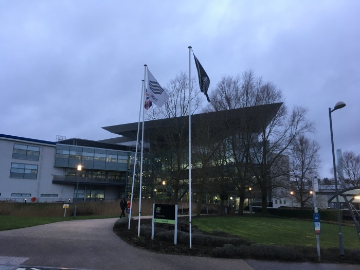
A while ago Mark (leader of the top secret project we are involved in) suggested that it had been a while since we visited the Met Office in Exeter where he works (blog tells me it was exactly 5 years ago, shortly after we had returned to the UK and before Blue Skies Research was really that well established). And then a few months later an invitation dropped through our letterbox for Malcolm’s birthday party. So, a cunning plan was hatched…we could travel down on Thursday, give seminars about our recently submitted papers (see previous posts here and here) on the Friday and stay for the Saturday party.
I always enjoy visiting the Met Office, it’s a hugely impressive place with a massive concentration of bright people working on interesting problems in the geosciences. Of course there must be some boring handle-turning in the day to day work and it’s a long way from just about everywhere. But Exeter is a nice enough place. Tickets and hotel were booked (not the Royal Clarence which has burnt down since our last trip) and the trip down was uneventful enough. Unfortunately Mark texted while we were on our way to say he was ill and was going home from work rather than meeting us for dinner that evening.
We got down in time for me to go for a short run in the fading light. The river seemed a bit high with all the recent rain.
I didn’t run along this side of the river where the path was submerged! There was a better path on the other side. And then on Friday morning, having scoped out the route through town, I managed to get a bit further along the river for sunrise.
Actually this particular bit is a canal.
We then had the (what we later discovered to be quintessentially Exonian) experience of seeing our bus vanish up the road a few minutes before we got to the stop at the scheduled time…fortunately there was enough time in hand to get to the Met Office. Mark was still absent but had already arranged a full day of activities with people to talk to.
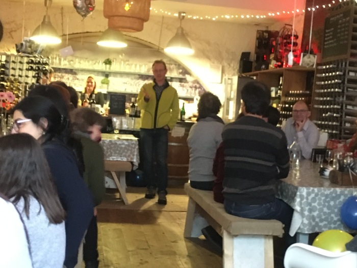
Seminars seemed to go ok, we gave a double-header with two fairly short talks summarising the two papers. Here and here are our pdfs if anyone is interested. I think there was also video streaming for people who couldn’t make it on the day, but probably no recording of this. It seems that a lot of people do a bit of working from home and/or part-time hours which is in principle a good thing though did mean there were a few absences.
By the end of the day we were quite tired from the unusual amount of talking – cats are a little less demanding! We are generally happy to work by ourselves on a day-to-day basis but it’s also great to have the occasional opportunity to bounce ideas around with people doing related work and we had a lot of interesting discussions.
Saturday was party day, and fortunately Storm Dennis passing over didn’t cause too many problems though I think a couple of attendees didn’t make it and it also meant the local parkrun was cancelled so we just mooched briefly through town in the morning. Of course we had seen the news of lots of rain and wind across the country and wondered if our trip home on Sunday would go smoothly.
Birthday boy above
I woke early on Sunday…and quickly found that there were almost no trains out of Exeter. Just one early train to London in fact, 2 hours earlier than our plan, so I quickly booked us onto it and we got to the station in plenty of time…to sit on the train for 20 minutes until they told us it wasn’t running after all and we would be offered a bus to Taunton instead. We briefly considered just going back to bed and staying an extra day but instead decided to take any option going in roughly the right direction and crossed our fingers, which in practice meant going to London and then out towards Leeds and amazingly managing to get home at the originally planned time. Train apps are a bit of a life-saver in these situations (also helpful with the train cancellations on our previous London trip) as it would have been rather more challenging to work out route options otherwise. I don’t really blame the train companies in these situations, there’s not a whole lot they can do about such a volume of rain in a short interval. It seems that the Exeter area was particularly badly hit this time and once out of the immediate vicinity, there was a reasonable service though at times it felt more like a cruise than a train journey!
Another new manuscript of ours out for review, this time on ESDD. The topic is as the title suggests. This work grew out of our trips to Hamburg and later Stockholm though it wasn’t really the original purpose of our collaboration. However, we were already working with a simple climate model and the 20th century temperature record when the Cox et al paper appeared (previous blogs here, here, here) so it seemed like an interesting and relevant diversion. Though the Cox et al paper was concerned with emergent constraints, this new manuscript doesn’t really have any connection to this one I blogged earlier though it is partly for the reasons explained in that post that I have presented the plots with S on the x-axis.
A fundamental point about emergent constraints, which I believe is basically agreed upon by everyone, is that it’s not enough to demonstrate a correlation between something you can measure and something you want to predict, you have to also present a reasonable argument why you expect this relationship to exist. With 10^6 variables to choose from in your GCM output (and an unlimited range of functions/combinations thereof) it is inevitable that correlations will exist, even in totally random data. So we can only reasonably claim that a relationship has predictive value if it has a theoretical foundation.
The use of variability (we are taking about the year-to-year variation in global mean temperature here after any trend has been removed) to predict sensitivity has a rather chequered history. Steve Schwartz tried and failed to do this, perhaps the clearest demonstration of this failure being that the relationship he postulated to exist for the climate system (founded on a very simple energy balance argument) did not work for the climate models. Cox et al sidestepped this pitfall by the simple and direct technique of presenting a relationship which had been directly derived from the ensemble of CMIP models, so by construction it worked for these. They also gave a reasonable-looking theoretical backing for the relationship, which was based on an analysis of a very simple energy balance argument. So on the face of it, it looked reasonable enough. Plenty of people had their doubts though as I’ve documented in the links above.
Rather than explore the emergent constraint aspect in more detail, we chose to approach the problem from a more fundamental perspective: what can we actually hope to learn from variability? We used the paradigm of idealised “perfect model” experiments, which enables us to generate very clear limits to our learning. The model we used is more-or-less the standard two layer energy balance of Winton, Held etc that has been widely adopted, but with a random noise term (after Hasselmann) added to the upper layer to simulate internal variability:
The single layer model that Cox et al used in their theoretical analysis is also recovered when the ocean mixing parameter γ is set to zero. So now the basic question we are addressing is, how accurately can we diagnose the sensitivity of this energy balance model, from analysis of the variability of its output?
Firstly, we can explore the relationship (in this model) between sensitivity S and the function of variability which Cox et al called ψ.
Focussing firstly on the fat grey dots, these represent the expected value of ψ from an unforced (ie, due entirely to internal variability) simulation of the single-layer energy balance model that Cox et al used as the theoretical foundation for their analysis. And just as they claimed, these points lie on a straight line. So far so good.
But…
It is well known that the single layer model does a pretty shabby job at representing GCM behaviour during the transient warming over the 20th century, and the two-layer version of the energy balance model gives vastly superior results for only a small increase in complexity. (This is partly why the Schwartz approach failed). Repeating our analysis with the two-layer version of the model, we get the black dots, where the relationship is clearly nonlinear. This model was in fact considered by the Cox group in a follow-up paper Williamson et al in which they argued that it still displayed a near-linear relationship between S and ψ over the range of interest spanned by GCMs. That’s true enough as the red line overlying the plot shows (I fitted that by hand to the 4 points in the 2-5C range) but there’s also a clear divergence from this relationship for larger values of S.
And moreover…
The vertical lines through each dot are error bars. These are the ±2 standard deviation ranges of the values of ψ that were obtained from a large sample of simulations, each simulation being 150 years long (a generous estimate of the observational time series we have available to deal with). It is very noticeable that the error bars grow substantially with S. This together with the curvature in the S-ψ relationship means that it is quite easy for a model with a very high sensitivity to generate a time series that has a moderate ψ value. The obvious consequence being that if you see a time series with a moderate ψ value, you can’t be sure the model that generated it did not have a high sensitivity.
We can use calculations of this type to generate the likelihood function p(ψ|S), which can be thought of as a horizontal slice though the above graph at a fixed value of ψ, and turn the handle of the Bayesian engine to generate posterior pdfs for sensitivity, based on having observed a given value of ψ. This is what the next plot shows, where the different colours of the solid lines refer to calculations which assumed observed values for ψ of 0.05, 0.1, 0.15 and 0.2 respectively.
These values correspond to the expected value of ψ you get with a sensitivity of around 1, 2.5, 5 and 10C respectively. So you can see from the cyan line that if you observe a value of 0.1 for ψ, that corresponds to a best estimate sensitivity of 2.5C in this experiment, you still can’t be very confident that the true value wasn’t rather a lot higher. It is only when you get a really small value of ψ that the sensitivity is tightly constrained (to be close to 1 in the case ψ=0.05 shown by the solid dark blue line).
The 4 solid lines correspond to the case where only S is uncertain and all other model parameters are precisely known. In the more realistic case where other model parameters such as ocean heat uptake are also somewhat uncertain, the solid blue line turns into the dotted line and in this case even the low sensitivity case has significant uncertainty on the high side.
It is also very noticeable that these posterior pdfs are strongly skewed, with a longer right hand tail than left hand (apart from the artificial truncation at 10C). This could be directly predicted from the first plot where the large increase in uncertainty and flattening of the S-ψ relationship means that ψ has much less discriminatory power at high values of S. Incidentally, the prior used for S in all these experiments was uniform, which means that the likelihood is the same shape as the plotted curves and thus we can see that the likelihood is itself skewed, meaning that this is an intrinsic property of the underlying model, rather than an artefact of some funny Bayesian sleight-of-hand. The ordinary least squares approach of a standard emergent constraint analysis doesn’t acknowledge or account for this skew correctly and instead can only generate a symmetric bell curve.
One thing that had been nagging away at me was the fact that we actually have a full time series of annual temperatures to play with, and there might be a better way of analysing them than to just calculate the ψ statistic. So we also did some calculations which used the exact likelihood of the full time series p({Ti}|S) where {Ti}, i = 1…n is the entire time series of temperature anomalies. I think this is a modest novelty of our paper, no-one else that I know of has done this calculation before, at least not quite in this experimental setting. The experiments below assume that we have perfect observations with no uncertainty, over a period of 150 years with no external forcing. Each simulation with the model generates a different sequence of internal variability, so we plotted the results from 20 replicates of each sensitivity value tested. The colours are as before, representing S = 1, 2.5 and 5C respectively. These results give an exact answer to the question of what it is possible to learn from the full time series of annual temperatures in the case of no external forcing.
So depending on the true value of S, you could occasionally get a reasonably tight constraint, if you are lucky, but unless S is rather low, this isn’t likely. These calculations again ignore all other uncertainties apart from S and assume we have a perfect model, which some might think just a touch on the optimistic side…
So much for internal variability. We don’t have a period of time in the historical record in which there was no external forcing anyway, so maybe that was a bit academic. In fact some of the comments on the Cox paper argued (and Cox et al acknowledged in their reply) that the forced response might be affecting their calculation of ψ, so we also considered transient simulations of the 20th century and implemented the windowed detrending method that they had (originally) argued removed the majority of the forced response. The S-ψ relationship in that case becomes:
where this time the grey and black dots and bars relate not to one and two layer models, but whether S alone is uncertain, or whether other parameters beside S are also considered uncertain. The crosses are results from a bunch of CMIP5 models that I had lying around, not precisely the same set that Cox et al used but significantly overlapping with them. Rather than just using one simulation per model, this plot includes all the ensemble members I had, roughly 90 model runs in total from about 25 models. There appears to be a vague compatibility between the GCM results and the simple energy balance model, but the GCMs don’t show the same flattening off or wide spread at high sensitivity values. Incidentally the set of GCM results plotted here don’t fit a straight line anywhere nearly as closely as the set Cox et al used. It’s not at all obvious to me why this is the case, and I suspect they just got lucky with the particular set of models they had combined with the specific choices they made in their analysis.
So it’s no surprise that we get very similar results when looking at detrended variability arising from the forced 20th century simulations. I won’t bore you with more pictures as this post is already rather long. The same general principles apply.
The conclusion is that the theory that Cox et al used to justify their emergent constraint analysis, actually refutes their use of a linear fit using ordinary least squares, because the relationship between S and ψ is significantly nonlinear and heteroscedastic (meaning the uncertainties are not constant but vary strongly with S). The upshot is that any constraint generated from ψ – or even more generally, any constraint derived from internal or forced variability – is necessarily going to be skewed with a tail to high values of S. However, variability does still have the potential to be somewhat informative about S and shouldn’t be ignored completely, which many analyses based on the long-term trend automatically do.
Nope, Can't be bothered. There's only a handful of posts for 2019, you can read them from the sidebar. Or just scroll down the page. I will be posting about real science quite soon though, once we have recovered from the insane 31 Dec IPCC deadline. Who thought that was a good idea? Bad enough to have that for our own paper, but then along came another couple that we were co-authors on, that required commenting and editing, and a project proposal for which there was really no reason at all for the same deadline to be picked, but back when we were first talking about it, it didn't seem to matter...
Anyway, all 4 things got done in time. Phew. Watch this space for further news.
At the start of the year I made some predictions. It's now time to see how I did.
In reverse order....
6. The level of CO2 in the atmosphere will increase (p=0.999).
Yup. I don't really need to wait for 1 Jan for that.
5. 2019 will be warmer than most years this century so far (p=0.75 - not the result of any real analysis).
As above, I know we've a few days to go but no need to wait for this one, which has been very clear for a good while now.
4. We will also submit a highly impactful paper in collaboration with many others (p=0.85).
Done, reviews back which look broadly ok, revision planned for early next year when we all have a bit of time (31 Dec is a stupid IPCC submission deadline for lots of other stuff).
3. Jules and I will finish off the rather delayed work with Thorsten and Bjorn (p=0.95).
Yes, the project is done, through the write-up continues. Actually we hope to submit a paper by 31 Dec but there will be more to do next year too.
2. I will run a time (just!) under 2:45 at Manchester marathon (p=0.6).
Nope, 2:47:15 this time. The prediction was made just a few days after I'd run a big PB in a 10k but even then I thought it was barely more likely than not, and it got less likely as the date approached.
1. Brexit won't happen (p=0.95).
On re-reading the old post, I have to admit I cannot remember the precise intention I had when I wrote this. Given the annual time frame of the remainder of the bets, and the narrative of that time being that we were certainly going to leave on the 29th March (as repeated over 100 times by May - remember her? - and the rest of them) I do believe I must have been referring to leaving during 2019. After all, I could never hope to validate a bet of infinite duration. So yes, I'm going to give myself this one.
On the other hand, I did actually think that we would probably not be stupid enough to leave at all, and clearly I misunderestimated the electorate and also the dishonesty of the Conservative Party, or perhaps as it should be known, the English National Party. I have learnt from that misjudgment and will not be offering any predictions as to where we end up at the end of next year. Which is sort of inconvenient, as we are trying to arrange a new contract with our European friends for work which could extend into 2021. Our options would seem to include: limiting the scope of the contract to what we can confidently complete strictly within 2020, which is far from ideal, or shifting everything to Estonia (incurring additional costs and inconvenience for us, though it may be the best option in the long term). Or just take a punt and cross our fingers that it all turns out ok, despite there being as yet no hint of a sketch of a plan as to how the sales of services into the EU will be regulated or taxed past 2020. It is quite possible that we'll just shut down the (very modest) operation and put our feet up. I'm still waiting for the brexiters to tell me how any of this is in the country's interests. But that's a rant for another day. Perhaps it's something to do with having enough of experts. As for scoring my predictions: the idea of a “proper scoring rule” is to provide a useful measure of performance for probabilistic prediction. A natural choice is the logarithmic scoring rule L = log(p) where p is the probability assigned to the outcome, and with all of my predictions having a binary yes/no basis I'll use base 2 for the calculation. The aim is to maximise the score (ie minimise its negativity, as the log of numbers in the range 0 to 1 is negative). A certain prediction where we assign a probability of p=1 to something that comes out right scores a maximum 0, a coin toss is -1 whether right or wrong but if you predict something to only have a p=0.1 chance and it happens, then the score is log(0.1) which in base 2 is a whopping -3.3. Assigning a probability of 0 to the event that happens is a bad idea, the score is infinitely negative...oops. My score is therefore: 0 - 0.42 - .23 - .07 -1.32 - .07 = 2.11 or about 0.35 per bet, which is equivalent to assigning p=0.78 to the correct outcome each time (which is just the geometric mean of the probabilities I did assign). Of course some were very easy, but that's why I gave them high p estimates which means high score (but a big risk if I'd got them wrong). I could have given a higher probability to the temperature prediction if I'd bothered thinking about it a bit more carefully. The running one was the only truly difficult prediction, because I was specifically calibrating the threshold to be close to the border of what I might achieve. It might have been better presented as a distribution for my finish time, where I would have had to judge the sharpness of the pdf as well as its location (ie mean).
There’s a new book just out "Contemporary Climate Change Debates: A Student Primer" edited by Mike Hulme. I contributed a short essay arguing the negative side of the above question. It was originally intended to be "Will exceeding 2C of warming lock the world onto a 'Hothouse Earth' trajectory?" but no-one could be found to argue in favour of that (this was shortly after the publication of the Steffen nonsense) so we settled on something a bit more vague. Maybe I should summarise my compelling argument but don’t have time right now so you’ll have to take my word for it.
I haven’t had time to read the book but my complementary copy just arrived (hence the post) and the table of contents is quite interesting, so maybe it would make a good Christmas present for the person who is interested in climate change – or even for someone who isn’t!
Introduction: Why and how to debate climate change
Mike Hulme
1. Is climate change the most important challenge of our times?
Sarah Cornell and Aarti Gupta
PART I: What do we need to know?
2. Is the concept of 'tipping point' helpful for describing and communicating possible climate futures?
Michel Crucifix and James Annan
3. Should individual extreme weather events be attributed to human agency?
Friederike E.L. Otto and Greg Lusk
4. Does climate change drive violence, conflict and human migration?
David D. Zhang and Qing Pei; Christiane Fröhlich and Tobias Ide
5. Can the social cost of carbon be calculated?
Reyer Gerlagh and Roweno Heijmans; Kozo Torasan Mayumi
PART II: What should we do?
6. Are carbon markets the best way to address climate change?
Misato Sato and Timothy Laing; Mike Hulme
7. Should future investments in energy technology be limited exclusively to renewables?
Jennie C. Stephens and Gregory Nemet
8. Is it necessary to research solar climate engineering as a possible backstop technology?
Jane C.S. Long and Rose Cairns
PART III: On what grounds should we base our actions?
9. Is emphasising consensus in climate science helpful for policymaking?
John Cook and Warren Pearce
10. Do rich people rather than rich countries bear the greatest responsibility for climate change?
Paul G. Harris and Kenneth Shockley
11. Is climate change a human rights violation?
Catriona McKinnon and Marie-Catherine Petersmann
PART IV: Who should be the agents of change?
12. Does successful emissions reduction lie in the hands of non-state rather than state actors?
Liliana B. Andronova and Kim Coetzee
13. Is legal adjudication essential for enforcing ambitious climate change policies?
Eloise Scotford; Marjan Peeters and Ellen Vos
14. Does the 'Chinese model' of environmental governance demonstrate to the world how to govern the climate?
Tianbao Qin and Meng Zhang; Lei Liu and Pu Wang
15. Are social media making constructive climate policymaking harder?
Mike S. Schäfer and Peter North
I believe the title of the post proclaims me to be an Estonian e-resident. jules likewise. This marks the culmination of a very straightforward on-line process which was remarkably painless right up to the moment that we had to attend the Estonian Embassy in London to pick up our identity cards in person, at which point we had to brave Britain’s creaking rail network.
The point of establishing e-residency is to be able to set up a business there, which will enable Blue Skies Research to remain seamlessly in the EU in the event of the UK ever managing to leave. Not that the latter looks very likely, but in order to collaborate on any long-term project based on EU funding we need to be able to prove that there’s a plan in place to cover the theoretical possibility. This must be one of these “Brexit bonus” things that the tories have been promising us for the past few years. Though “bonus” would usually imply some sort of gain rather than added costs and bureaucracy, not to mention the losses in corporation tax which will henceforth be paid in Estonia rather than the UK. Even for our part-time hobby business, that is likely to be several thousands, perhaps up to ten thousand pounds, per year lost to the UK indefinitely into the future. Our combined share of EU membership fees is probably under a hundred quid per year. Even the bare cost of health insurance for when we visit our colleagues there will cost more than that when we lose the EHIC. But we will apparently get blue passports and we may eventually get a new 50p piece too when they have worked out the design. Apparently they had almost finalised that a while back, but hadn't worked out what to do about the border. Boom tish. Of course they still haven't, so Bonson is just lying through his teeth every time he opens his mouth, and the same old tory voters will just lap it up cos he's such a cheeky chappy with those clever latin bons mots.
We did managed to arrange another couple of things during the two-day trip, so it wasn’t a total waste of time. And it was cheaper than expected too, due to three of the four train trips being significantly delayed to such an extent we can reclaim half of the travel costs.
Just had a couple of weeks in Stockholm, courtesy of Thorsten Mauritsen at MISU. who we had previously visited in Hamburg. Lots of science will be forthcoming but we are too busy doing it to write about it for now
For the moment, I will just note that Thorsten is Danish, previously working in Germany but now in Sweden, we had discussions with his British and French group members, the Head of Department is Spanish. Discussions in the canteen seemed to be mostly English in a variety of accents (including the Dutch student who had considered coming to the UK but who had been dissuaded by the obvious reason), mixed with a range of unidentifiable Scandinavian languages – presumably mostly, if not all, Swedish. Theresa May and Jeremy Corbyn would be horrified to hear of such an outrageous situation and I’m relieved that they are doing their level best to ensure that no Brits will risk encountering such a terrible situation again.
(Actually, to be honest I am relieved that their level best is so pitiful that we aren’t actually going to leave the EU. But I’m still disgusted that they are so scared at the thought of people living, working and studying in different countries that they are completely fixated on the idea of preventing us from doing so.)
Haga parkrun was close to our hotel, and by strange quirk of fate on Sunday morning I ran a route which quite closely approximates a lap of the upcoming Stockholm marathon. I hadn't even known there was a marathon. Some were out practising for the famous Stockholm ski marathon too.
Stockholm has a lot of islands, and as a result, there’s a lot of coastline and water.
On our last night we had dinner in a Michelin-starred restaurant which was an interesting experience. However this photo below is just the little castle on the top of Kastellholmen which may be used as some sort of conference centre I think.




 But readers can make up their own minds as to how generally applicable it is. It’s an idea, not a law.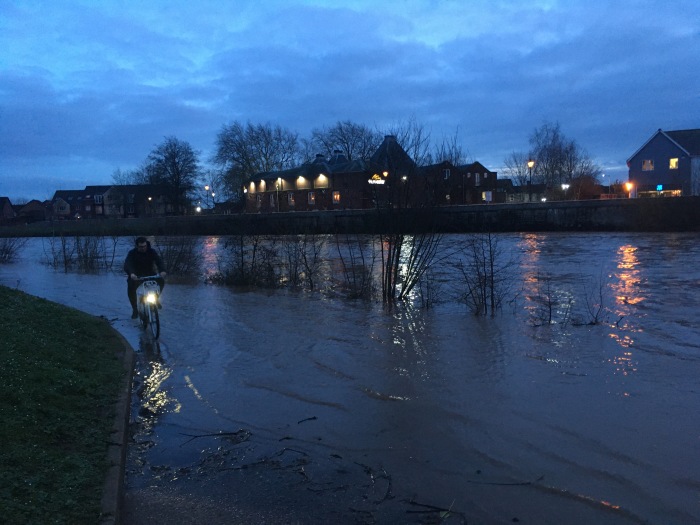



 On our last night we had dinner in a Michelin-starred restaurant which was an interesting experience. However this photo below is just the little castle on the top of Kastellholmen which may be used as some sort of conference centre I think.
