The new study from IC

I haven't had time to examine this new research in great detail but it looks pretty good to me (maybe one or two minor caveats). They have fitted a fairly simple mechanistic statistical model to time series data for deaths in a large number of European countries, using a Bayesian hierarchical modelling approach to estimate the effects of various "non-pharmaceutical interventions" like shutting schools and banning large meetings which have been widely adopted. I suspect (could be wrong tho) that the reason for using a primarily statistical model is that it's quicker and easier for their method than a fully dynamical model like the one I'm using. They say it is fundamentally similar to SIR though, so I don't think their results should be any the worse for it (though perhaps the E box makes a difference?).

First and foremost, by far the most significant result IMO is that they find the initial R0 to be much larger than in the complex mechanistic modelling of Ferguson et al. This confirms what I suggested a few days ago, which was based on the fact that their value of R0 = 2.4 (ish) was simply not compatible with the rapid exponential growth rate in the UK and just about everywhere else in the western world.

Here are pics of their values for a number of countries, for their preferred reproductive time scale of 6.5 days. Left is prior to interventions, right is current post-intervention estimates.

 

You may spot that all the values on the right imply a substantial probability of R0 > 1, as I also suggested in my recent post. If the initial R0 is high, it's hard to reduce it enough to get it below 1. If true, that would mean ongoing growth of the epidemic, albeit at a lower rate and with a longer lower peak than would be the case without the interventions. I will show over the next few days what the implications of this could be over the longer term.

It's also important to realise that these values on the right depend on the data for all countries - this is the "hierarchical" bit - there is no evidence from the UK data itself of any significant drop in R, as you can work out from the below plot which gives the fit and a one-week forecast. There simply hasn't been long enough since the restrictions were put in place, for anything to feed through into the deaths. Though if it bends in the near future, that will be a strong indication that something is going on. They appear to be 3 days behind reality here - it looks like they haven't got the two small drops and most recent large rise.

Despite my best intentions, I don't really see much to criticise, except that they should have done this a week or two ago before releasing the complex modelling results in which they made such poor parameter choices. Obviously, they would not have been able to estimate the effect of interventions using this method, but they'd have got the initial growth rate right.

It's a little like presenting forecasts from one of the new CMIP6 models, without checking that it has roughly the right warming rate over the last few decades. You'd be better off using an energy balance that was fitted to recent history, especially if you were primarily interested in the broad details such as large-scale temperature trend. In fact that's a pretty direct analogy, except that the epidemic model is much simpler and more easily tuned than a state of the art climate model. Though they also had a bit less time to do it all :-)

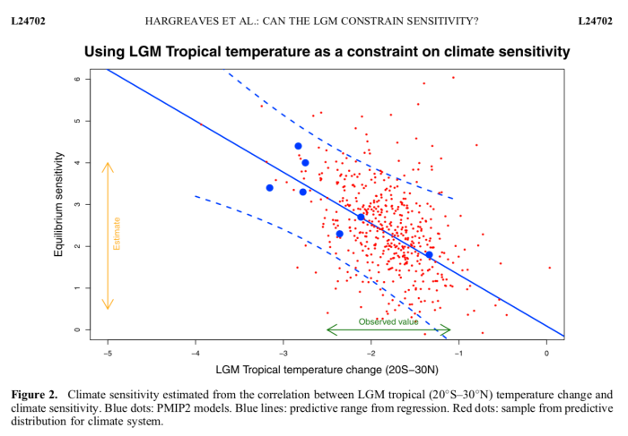
As for the caveats however - I had to laugh at this, especially the description above:

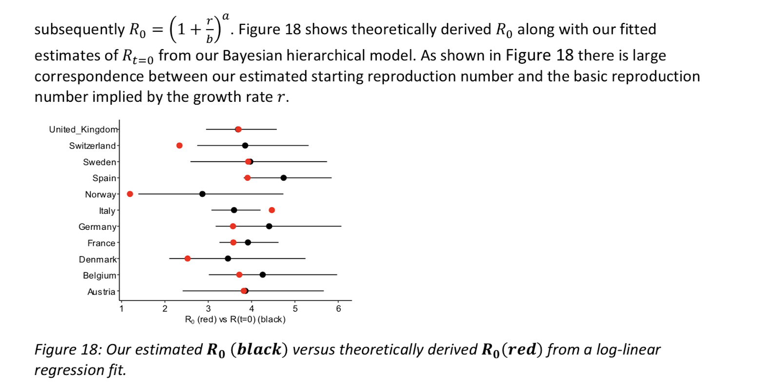
I remember seeing a similarly impressive "large correspondence" plotted in a climate science paper a while back. I pressed the authors for the correlation between the two sets of data, and they admitted there wasn't one.

But that's a minor quibble. It's a really interesting piece of work.

I am now just about in a position to show results from my attempts at doing proper MCMC fits to time series data with the SEIR model so it will be interesting to see how the results compare. This can also give longer-term forecasts (under various scenario assumptions of course).

BlueSkiesResearch.org.uk: How to do emergent constraints properly

Way back in the mists of time, we did a little bit of work on "emergent constraints". This is a slightly hackneyed term referring to the use of a correlation across an ensemble of models between something we can’t measure but want to estimate (like the equilibrium climate sensitivity S) and something that we can measure like, say, the temperature change T that took place at the Last Glacial Maximum….

Actually our early work on this sort of stuff dates back 15 years but it was a bit more recently, in 2012 when we published this result

in the paper blogged about here that we started to think about it a little more carefully. It is easy to plot S against T and do a linear regression, but what does it really mean and how should the uncertainties be handled? Should we regress S on T or T on S? [I hate the arcane terminology of linear regression, the point is whether S is used to predict T (with some uncertainty) or T is used to predict S (with a different uncertainty)]. We settled for the conventional approach in the above picture, but it wasn’t entirely clear that this was best.

And is this regression-based approach better or worse than, or even much the same as, using a more conventional and well-established Bayesian Model Averaging/Weighting approach anyway? We raised these questions in the 2012 paper and I’d always intended to think about it more carefully but the opportunity never really arose until our trip to Stockholm where we met a very bright PhD student who was interested in paleoclimate stuff and shortly afterwards attended this workshop (jules helped to organise this: I don’t think I ever got round to blogging it for some reason). With the new PMIP4/CMIP6 model simulations being performed, it seemed a good time to revisit any past-future relationships and this prompted us to reconsider the underlying theory which has until now remained largely absent from the literature.

So, what is new our big idea? Well, we approached it from the principles of Bayesian updating. If you want to generate an estimate of S that is informed by the (paleoclimate) observation of T, which we write as p(S|T), then we use Bayes Theorem to say that

p(S|T) ∝ p(T|S)p(S).

Note that when using this paradigm, the way for the observations T to enter in to the calculation is via the likelihood p(T|S) which is a function that takes S as an input, and predicts the resulting T (probabilistically). Therefore, if you want to use some emergent constraint quasi-linear relationship between T and S as the basis for the estimation then it only really makes sense to use S as the predictor and T as the predictand. This is the opposite way round to how emergent constraints have generally (always?) been implemented in practice, including in our previous work.

So, in order to proceed, we need to create a likelihood p(T|S) out of our ensemble of climate models (ie, (T,S) pairs). Bayesian linear regression (BLR) is the obvious answer here – like ordinary linear regression, except with priors over the coefficients. I must admit I didn’t actually know this was a standard thing that people did until I’d convinced myself that this must be what we had to do, but there is even a wikipedia page about it.

This therefore is the main novelty of our research: presenting a way of embedding these empirical quasi-linear relationships described as "emergent constraints" in a standard Bayesian framework, with the associated implication that it should be done the other way round.

Given the framework, it’s pretty much plain sailing from there. We have to choose priors on the regression coefficients – this is a strength rather than a weakness in my view, as it forces us to explicitly consider whether we consider the relationship to be physically sound, and argue for its form. Of course it’s easy to test the sensitivity of results to these prior assumptions. The BLR is easy enough to do numerically, even without using the analytical results that can be generated for particular forms of priors. And here’s one of the results in the paper. Note that unlabelled x-axis is sensitivity in both of these plots, in contrast to being the y-axis in the one above.

While we were doing this work, it turns out that others had also been thinking about the underlying foundations of emergent constraints, and two other highly relevant papers were published very recently. Bowman et al introduces a new framework which seems to be equivalent to a Kalman Filter. In the limit of a large ensemble with a Gaussian distribution, I think this is also equivalent to a Bayesian weighting scheme. One aspect of this that I don’t particularly like is the implication that the model distribution is used as the prior. Other than that, I think it’s a neat idea that probably improves on the Bayesian weighting (eg that we did in the 2012 paper) in the typical case that we have where the ensemble is small and sparse. Fitting a Gaussian is likely to be more robust than using a weighted sum of a small number of samples. But, it does mean you start off from the assumption that the model ensemble spread is a good estimator for S, which is therefore considered unlikely to like outside this range. Whereas regression allows us to extrapolate, in the case where the observation is at our outside the ensemble range.

The other paper by Williamson and Sansom presented a BLR approach which is in many ways rather similar to ours (more statistically sophisticated in several aspects). However, they fitted this machinery around the conventional regression direction. This means that their underlying prior was defined on the observation with S just being an implied consequence. This works ok if you only want to use reference priors (uniform on both T and S) but I’m not sure how it would work if you already had a prior estimate of S and wanted to update that. Our paper in fact shows directly the effect of using both LGM and Pliocene simulations to sequentially update the sensitivity.

The limited number of new PMIP4/CMIP6 simulations means that our results are substantially based on older models, and the results aren’t particularly exciting at this stage. There’s a chance of adding one or two more dots on the plots as the simulations are completed, perhaps during the review process depending how rapidly it proceeds. With climate scientists scrambling to meet the IPCC submission deadline of 31 Dec, there is now a huge glut of papers needing reviewers…

Implicit priors and the energy balance of the earth system

So, this old chestnut seems to keep on coming back....

Back in 2002, Gregory et al proposed that we could generate “An observationally based estimate of the climate sensitivity” via the energy balance equation S = F_2x dT/Q where S is the equilibrium sensitivity to 2xCO2, F_2x = 3.7 is the (known constant) forcing of 2xCO2, dT is the observed surface air temperature change and Q is the net radiative imbalance at the surface which takes account of both radiative forcing and the deep ocean heat uptake. (Their notation is marginally different, I'm simplifying a bit.)

Observational values for both dT and Q can be calculated/observed, albeit with uncertainties (reasonably taken to be Gaussian). Repeatedly sampling from these observationally-derived distributions and taking the ratio generates an ensemble of values for S which can be used as a probability distribution. Or can it? Is there a valid Bayesian interpretation of this, and if so, what was the prior for S? Because we know that it is not possible to generate a Bayesian posterior pdf from observations alone. And yet, it seems that one was generated.

This method may date back to before Gregory et al, and is still used quite regularly. For example, Thorsten Mauritsen (who we were visiting in Hamburg recently) and Robert Pincus did it in their recent “Committed warming” paper. Using historical observations, they generated a rather tight estimate for S as 1.1-4.4C, though this wasn't really the main focus of their paper. It seems a bit optimistic compared to much of the literature (which indicates the 20th century to provide a rather weaker constraint than that) so what's the explanation for this?

The key is in the use of the observationally-derived distributions for the quantities dT and Q. It seems quite common among scientists to interpret a measurement x_o of an unknown x, with some known (or perhaps assumed) uncertainty σ, as implying the probability distribution N(x_o,σ) for x. However, this is not justifiable in general. In Bayesian terms, it may be considered equivalent to starting with a uniform prior for x and updating with the likelihood arising from the observation. In many cases, this may be a reasonable enough thing to do, but it's not automatically correct. For instance, if x is known to be positive definite, then the posterior distribution must be truncated at 0, making it no longer Gaussian (even if only to a negligible degree). (Note however that it is perfectly permissible to do things like use (x_o - 2σ, x_o + 2σ) as a 95% frequentist confidence interval for x, even when it is not a reasonable 95% Bayesian credible interval. Most scientists don't really understand the distinction between confidence intervals and credible intervals, which may help to explain why the error is so prevalent.)

So by using the observational estimates for dT and Q in this way, the researcher is implicitly making the assumption of independent uniform priors for these quantities. This implies, via the energy balance equation, that their prior on S is the quotient of two uniform priors. Which has a funny shape in general, with a flat region near 0 and then a quadratically-decaying tail. Moreover, this prior on S is not independent of the prior for either dT or Q. Although it looks like there are three unknown quantities, the energy balance equation tying them together means there are only two degrees of freedom here.

At the time of the IPCC AR4, this rather unconventional implicit prior for S was noticed by Nic Lewis who engaged in some correspondence with IPCC authors about the description and presentation of the Gregory et al results in that IPCC report. His interpretation and analysis is very sightly different to mine, in that he took the uncertainty in dT to be so (relatively) small that one could ignore it and consider the uniform prior on Q alone, which implies an inverse quadratic prior on S. However the principle of his analysis is similar enough.

In my opinion, a much more straightforward and natural way to approach the problem is instead to define the priors over Q and S directly. These can be whatever we want and are prepared to defend publicly. I've previously advocated a Cauchy prior for S which avoids the unreasonableness and arbitrariness of a uniform prior for this constant. In contrast, a uniform prior over Q (independent of S) is probably fairly harmless in this instance, and this does allow for directly using the observational estimate of Q as a pdf. Sampling from these priors to generate an ensemble of (S,Q) pairs allows us to calculate the resulting dT and weight the ensemble members according to how well the simulated values match the observed temperature rise. This is standard Monte Carlo integration using Bayes Theorem to update a prior with a likelihood. Applying this approach to Thorsten's data set (and using my preferred Cauchy prior), we obtain a slightly higher range for S of 1.2 - 4.8C. Here's a picture of the results (oops, ECS = S there, an inconsistent labelling that I can't be bothered fixing).

The median and 5-95% ranges for prior and posterior are also given. As you can see, the Cauchy prior doesn't really cut off the high tail that aggressively. In fact it's a lot higher than a U[0,10] or even U[0,20] prior would imply.  

More on Bayesian approaches to detection and attribution

Timely given events all over the place, this new paper by Mann et al has just appeared.  It's a well-aimed jab at the detection and attribution industry which could perhaps be held substantially responsible for the sterile “debate” over the extent to which AGW has influenced extreme events (and/or will do so in the future). I've argued against D&A several times in the past (such as here, here, here and here) and don't intend to rehash the same arguments over and over again. Suffice to say that it doesn't usefully address the questions that matter, and cannot do so by design.

Mann et al argue that the standard frequentist approach to D&A is inappropriate both from a simple example which shows it to generate poor results, and from the ethical argument that “do no harm” is a better starting point than “assume harmless”. The precautionary versus proactionary principles can be argued indefinitely, and neither really works when reduced ad absurdum, so I'm not really convinced that the latter is a strong argument. A clearer demonstration could perhaps have been provided by a rational cost-benefit analysis in which costs of action versus inaction (and the payoffs) could have been explicitly calculated. This would have still supported their argument of course, as the frequentist approach is not a rational basis for decisions. I suppose that's where I tend to part company with the philosophers (check the co-author list) in preferring a more quantitative approach. I'm not saying they are wrong, it's perhaps a matter of taste.

[I find to my surprise I have not written about the precautionary vs proactionary principle before]

Other points that could have been made (and had I been a reviewer, I'd probably have encouraged the authors to include them) are that when data are limited and the statistical power of the analysis is weak, it is not only inevitable that any frequentist-based estimate that achieves statistical significance will be a large overestimate of the true magnitude of the effect, but there's even a substantial chance it will have the wrong sign! A Bayesian prior solves (or at least greatly ameliorates) these problems. Another benefit of the Bayesian approach is the ability to integrate different sources of information. My favourite example of the weakness of traditional D&A here is the way that we can (at least this was the case a few years ago) barely “attribute” any warming of the world's oceans under this methodology. The reason for this is that the internal variability of the oceans is large (and uncertain) enough that we cannot be entirely confident that an unforced ocean would not have warmed up by itself. On the other hand, it is absurd to believe the null hypothesis that we haven't warmed it, as it has been in contact with the atmosphere that we have certainly warmed, and the energy imbalance due to GHGs is significant, and we've even observed a warming very closely in line with what our models predict should have happened. But D&A can't assimilate this information. In the context of Mann et al, we might consider information about warming sea surface temperatures as relevant to diagnosing and predicting hurricanes, for example, rather than relying entirely on storm counts.

BlueSkiesResearch.org.uk: The future of climate science

The future of climate science

Posted: 24 Sep 2014 09:08 AM PDT

I recently had the pleasure of a trip to Brussels, courtesy of this workshop, organised by Michel Crucifix, Valerio Lucarini and Stéphane Vannitsem. Titled "Advances in Climate Theory", it was a chance to discuss ideas related to…advances in climate theory, surprisingly enough. In practice, that included lots about the dynamics of the wiggles that are seen in paleoclimate cores (are they noise-induced or due to an inherent instability?), various nonlinearities, some entropy stuff which (deservedly?!) got a bit of rough ride from the audience. My talk was not so much on theory as practice, that is, the practical aspects of using the past to improve predictions of the future.

We were based in the Royal Meteorological Institute, which was a nice site some way out of town (walkable from the hotel, which was great apart from the day we had a brief downpour of biblical proportions just as I sneaked out a little bit early). Here is a picure of Michel orating on dynamical things…

It wasn’t all fun though – on my first night I had to forage on my own and only found some gueueuze for dinner, along with geueze-flavoured pate.

Beer is the answer – it doesn’t matter what the question is.

Objective probability or automatic nonsense?

A follow-up to the previous probability post.

Perhaps this will provide a clearer demonstration of the limitations of Nic's method. In his post, he conveniently provided a simple worked example, which in his view demonstrates how well his method works. A big advantage of using his example is that hopefully no-one can argue I've misapplied his method :-) This is Figure 2 from his post:

This example is based on carbon-14 dating, about which I know very little, but hopefully enough to explain what is going on. The x-axis in the above is real age with 0 corresponding to the "present day", which I think is generally defined as 1950 (so papers don't need to be continually reparsed as time passes). The y-axis is "carbon age" which is basically a measure of the C14 content of something under investigation, typically something organic (plant or animal). The basic idea is that the plant or aminal took up C14 as it grew, but this C14 slowly decays so the proportion in the sample declines after death according to the C14 half-life. So in principle you would think that the age (at death) can be determined directly from measurement of the proportion of carbon that is C14. However, the proportion of C14 in the original organism depends on the ambient concentration of C14 which has varied significantly in the past (it's created by cosmic rays and the like), so there's quite a complicated calibration curve. The black line in the above is a simplified and stylised version of what a curve could look like (Nic's post also has a real calibration curve, but this example is clearer to work with).

So in the example above, the red gaussian represents a measurement of radiocarbon which represents a "carbon age" of about 1000y, with some uncertainty. This is mapped via the calibration curve into a real age distribution on the x-axis, and Nic has provided two worked examples using a uniform prior and his favoured Jeffreys prior.

As some of you may recall, I lived in Japan until recently. Quite by chance, my home town of Kamakura was the capital of Japan for a brief period roughly 7-800y ago. Lots of temples date from that time, and there are numerous wooden artefacts which are well-dated to the Kamakura Era (let's assume, carved out of conteporaneous wood, though of course wood is generally a bit older than the date of the tree felling). Let's see what happens when we try to carbon-date some of these artefacts using Nic's method.

Well, one thing that Nic's method will say with certainty is "this is not a Kamakura-era artefact"! The example above is a plausible outcome, with the carbon age of 1000y covering the entire Kamakura era. Nic's posterior (green solid curve) is flatlining along the axis over the range 650-900y, meaning zero probability for this whole range. The obvious reason for this is that his prior (dashed line) is also flatlining here, making it essentially impossible for any evidence, no matter how strong, to overturn the prior presumption that the age is not in this range.

It is important to recognise that the problem here is not with the actual measurement itself. In fact the measurement shown in the figure indicates very high likelihood (in the Bayesian sense) of the Kamakura era. The problem is entirely in Nic's prior, which ruled out this time interval even before the measurement was made - just because he knew that a measurement of carbon age was going to be made!

Nic uses the emotionally appealing terminology of "objective probability" for this method. I don't blame him for this (he didn't invent it) but I do wonder whether many people have been seduced by the language without understanding what it actually does. You can see Richard Tol insisting that the Jeffreys prior is "truly uninformative" in a comment on my previous post, for example. Well, that might be true, but only if you define "uninformative" in a technical sense not equivalent to common english usage. If you then use it in public, including among scientists who are not well versed in this stuff, then people are going to get badly misled. Frame and Allen went down this rabbit hole a few years ago, I'm not sure if they ever came out. It seems to work for many as an anchoring point, when you discuss in detail, they acknowledge that yes, it's not really "uninformative" or "ignorant" really, but then they quickly revert back to this usage, and the caveats somehow get lost.

I propose that it would be better to use the term "automatic" rather than "objective". What Nic is presenting is an automatic way of generating probabilities, though it remains questionable (to put it mildly) whether they are of any value. Nic's method insists that no trace remains of the Kamakura era, and I don't see any point in a probabilistic method that generates such obvious nonsense.

Coverage

Or, why Nic Lewis is wrong.

Long time no post, but I've been thinking recently about climate sensitivity (about which more soon) and was provoked into writing something by this post, in which Nic Lewis sings the praises of so-called "objective Bayesian" methods.

Firstly, I'd like to acknowledge that Nic has made a significant contribution to research on climate sensitivity, both through identifying a number of errors in the work of others (eg here, here and most recently here) and through his own contributions in the literature and elsewhere. Nevertheless, I think that what he writes about so-called "objective" priors and Bayesian methods is deeply misleading. No prior can encapsulate no knowledge, and underneath the use of these bold claims there is always a much more mealy-mouthed explanation in terms of a prior having "minimal" influence, and then you need to have a look at what "minimal" really means, and so on. Well, such a prior may or may not be a good thing, but it is certainly not what I understand "no information" to mean. I suggest that "automatic" is a less emotive term than "objective" and would be less likely to mislead people as to what is really going on. Nic is suggesting ways of automatically choosing a prior, which may or may not have useful properties.

[As a somewhat unrelated aside, it seems strange to me that the authors of the corrigendum here concerning a detail of the method, do not also correct their erroneous claims concerning "ignorant" priors. It's one thing to let errors lie in earlier work - no-one goes back and corrects minor details routinely - but it is unfortunate that when actually writing a correction about something they state does not substantially affect their results, they didn't take the opportunity to also correct a horrible error that has seriously mislead much of the climate science community and which continues to undermine much work in this area. I'm left with the uncomfortable conclusion that they still don't accept that this aspect of the work was actually in error, despite my paper which they are apparently trying to ignore rather than respond to. But I'm digressing.]

All this stuff about "objective priors" is just rhetoric - the term simply does not mean what a lay-person might expect (including a climate scientist not well-versed in statistical methodology). The posterior P(S|O) is equal to to the (normalised) product of prior and likelihood - it makes no more sense to speak of a prior not influencing the posterior, as it does to talk of the width of a rectangle not influencing its area (= width x height). Attempts to get round this by then footnoting a vaguer "minimal effect, relative to the data" are just shifting the pea around under the thimble.

In his blog post, Nic also extolls the virtue of probabilistic coverage as a way of evaluating methods. This initially sounds very attractive - the idea being that your 95% intervals should include reality, 95% of the time (and similarly for other intervals). There is however a devil in the detail here, because such a probabilistic evaluation implies some sort of (infinitely) repeated sampling, and it's critical to consider what is being sampled, and how. If you consider only a perfect repetition in which both the unknown parameter(s) and the uncertain observational error(s) take precisely the same values, then any deterministic algorithm will return the same answer, so the coverage in this case will be either 100% or 0%! Instead of this, Nic considers repetition in which the parameter is fixed and the uncertain observations are repeated. Perfect coverage in this case sounds attractive, but it's trivial to think of examples where it is simply wrong, as I'll now present.

Let's assume Alice picks a parameter S (we'll consider her sampling distribution in a minute) and conceals it from Bob. Alice also samples an "error" e from the simple Gaussian N(0,1). Alice provides the sum O=S+e to Bob, who knows the sampling distribution for e. What should Bob infer about S? Frequentists have a simple answer that does not depend on any prior belief about S - their 95% confidence interval will be (S-2e,S+2e) (yes I'm approximating negligibly throughout the post). This has probabilistically perfect coverage if S is held fixed and e is repeatedly sampled. Note that even this approach, which basically every scientist and statistician in the world will agree is the correct answer to the situation as stated, does not have perfect coverage if instead e is held fixed and S is repeatedly sampled! In this case, coverage will be 100% or 0%, regardless of the sampling distribution of S. But never mind about that.

As for Bayesians, well they need a prior on S. One obvious choice is a uniform prior and this will basically give the same answer as the frequentist approach. But now let's consider the case that Alice picks S from the standard Normal N(0,1), and tells Bob that she is doing so. The frequentist interval still works here (i.e., ignoring this prior information about S), but Bayesian Bob can do "better", in the sense of generating a shorter interval. Using the prior N(0,1) - which I assert is the only prior anyone could reasonably use - his Bayesian posterior estimate for S is the Normal N(O/2,0.7), giving a 95% probability interval of (O/2-1.4,O/2+1.4). It is easy to see that for a fixed S, and repeated observational errors e, Bob will systematically shrink his central estimates towards the prior mean 0, relative to the true value of S. Let's say S=2, then (over a set of repeated observations) Bob's posterior estimates will be centred on 1 (since the mean of all the samples of e is 0) and far more than 5% of his 95% intervals (including the full 27% of cases where e is more negative than -0.6) will fail to include the true value of S. Conversely, if S=0, then far too many of Bob's 95% intervals will include S. In particular, all cases where e lies in (-2.8,2.8) - which is about 99.5% of them - will generate posteriors that include 0. So coverage - or probability matching, as Nic calls it - varies from far too generous, when S is close to 0, to far too rare, for extreme values of S.

I don't think that any rational Bayesian could possibly disagree with Bob's analysis here. I challenge Nic to present any other approach, based on "objective" priors or anything else, and defend it as a plausible alternative to the above. Or else, I hope he will accept that probability matching is simply not (always) a valid measure of performance. These Bayesian intervals are unambiguously and indisputably the correct answer in the situation as described, and yet they do not provide the correct coverage conditional on a fixed value for S

Just to be absolutely clear in summarising this - I believe Bayesian Bob is providing the only acceptable answer given the information as provided in this situation. No rational person could support a different belief about S, and therefore any alternative algorithm or answer is simply wrong. Bob's method does not provide matching probabilities, for a fixed S and repeated observations. Nothing in this paragraph is open to debate.

Therefore, I conclude that matching probabilities (in this sense, i.e. repeated sampling of obs for a fixed parameter) is not an appropriate test or desirable condition in general. There may be cases where it's a good thing, but this would have to be argued for explicitly.

The null hypothesis in climate science

Three papers have just appeared in WIREs Climate Change (here, here and here) discussing the role of the null hypothesis in climate science, especially detection and attribution.

Trenberth argues that, since the null (that we have not changed the climate) is not true, we should try to test some other null hypothesis. He sounds like someone who has just discovered that the frequentist approach is actually pretty useless in principle (as I've said many times before, it is fundamentally incapable of even addressing the questions that people want answers to), but although he seems to be grasping towards a Bayesian approach, he hasn't really got there, at least not in a coherent and clear manner. Curry is just nonsense as usual, and beside noting that she has (1) grossly misrepresented the IAC report and (2) abjectly failed to back up the claims that Curry and Webster made in a previous paper, there isn't really anything meaningful to discuss in what she said.

Myles Allen's commentary is by some distance the best of the bunch, in fact I broadly agree (shock horror) with what he has said. If one is going to take a frequentist approach, the null hypothesis of no effect is often an entirely reasonable starting point. It is important to understand that rejecting the null does not simply mean learning that there has been some effect, but it also indicates that we know (at least at some level of confidence) the direction of the effect! That is, it is not only an effect of zero which is rejected, but all possible negative (say) effects of any magnitude too - this generalisation may not be strictly correct in all possible applications of this sort of methodology, but I'm pretty sure it is true in practice for the D&A field. Especially when we are talking about the local incidence of extreme weather, there really are many cases when we have little reason for a prior belief in an anthropogenically-forced increase versus a decrease in these events, so a reasonable Bayesian approach would also start from a prior which was basically symmetric around zero. The correct interpretation of a non-rejection of the null here is not "there has been no effect" but rather "we don't know if AGW is making these events more or less likely/large". Much of Trenberth's complaint could be more productively aimed at the routine misinterpretation of D&A results, rather than the method of their generation. Trenberth also sometimes sounds like he is arguing that we should always assume that every bad thing was caused by (or at least exacerbated by) AGW, but this simply isn't tenable. Even if storminess increases in general, changes in storm tracks might lead to reduction in events in some areas, with Zahn and von Storch's work on polar lows an obvious example of this. On the other hand, there are also some types of event where we may have decent prior belief in the nature of the anthropogenically-forced change (such as temperature extremes) and in these cases it would be reasonable for a Bayesian to use a prior that reflects this belief.

I can find one thing to object to in Myles' commentary though, and that's the manner in which he tries to pre-judge the "consensus" response to Trenberth's argument. Noting that he (Allen) is in fact a major figure in forming the "consensus" in these private meetings where the handful of IPCC authors decide what to say, it sounds to me rather like a pre-emptive strike against anyone who might be tempted to take the opposing view. I would prefer it if he restricted himself to arguing on the basis of the issues rather than that he holds/forms the majority view. His behaviour here is reminiscent of the way he (and others) tried to reject our arguments about uniform priors, on the basis that everyone had already agreed that his approach was the correct solution. All that achieved was to slow the progress of knowledge by a few years.

Solution to the paradox of climate sensitivity

A lot of bloggable papers have suddenly appeared, so I will work through them over the next few days.

First, a quick comment about this interesting paper: "Solution to the paradox of climate sensitivity" by Salvador Pueyo. In it, he argues that we should use a log-uniform prior for estimating climate sensitivity. This is fundamentally an "Objective Bayes" approach, that "non-informative" can be interpreted in a unique way. I don't much like this point of view, but if one is going to take it, then it should at least be done properly, and he seems to have provided decent arguments in that direction. Readers may recall that IPCC authors have in the past claimed that a uniform distribution was the unique correct representation of ignorance, which formed one of the planks of their assessment of the literature in the AR4.

As we showed here, all this talk of a long tail basically vanishes when anything other than a uniform prior is used, so in that sense this new paper is broadly compatible with our existing results which were based on a subjective paradigm. However, I'm not sure how it would work with a more complex multivariate approach, as has been common in this sort of work (eg simultaneously considering the three major uncertainties of ocean heat uptake, aerosol forcing and sensitivity).

What the new IPCC authors will make of it all is anyone's guess. Perhaps we will find out in December some time, when the first draft is scheduled to be opened for comments.

Priors and climate sensitivity again

Several people have email about this article. I don't have anything particularly novel or interesting to say, so I'll just repeat an email that I sent regarding it...

---

From my point of view, the problem is not particularly in the treatment of the Forster and Gregory result - the authors had already in that paper pointed to the choice of prior as an important factor in the specific results they generated. More, the error was in the IPCC's endorsement and rigid adherence to the use of uniform prior, despite the existence of very straightforward arguments that this approach is simply not tenable:

http://www.springerlink.com/content/7np5t35mq27p3q24/
(also here:
http://www.jamstec.go.jp/frsgc/research/d5/jdannan/probrevised.pdf )

These arguments (which as you saw I made during the IPCC review process [here here here]) were basically brushed aside. The IPCC authors exclusively relied on and highlighted the results that had been generated using uniform priors, and downplayed alternative results, which already existed in the literature, that had been generated with different priors.

However, with the passage of time I believe my arguments have now become more widely (if grudgingly) accepted, so I look forward with some interest to see how the IPCC authors deal with the subject this time.

---

I should also add that I'm not at all convinced by the author's claims that a prior which is uniform in feedback (1/sensitivity) is "correct", rather, it is something that people have to think about, and may reasonably disagree. Such is life. It is theoretically possible that someone could even present a plausible argument for a uniform prior in sensitivity, but I've not yet seen one...

Statistically significant

Apparently global warming is statistically significant again.

But we all know that the difference between "significant" and not significant is not itself statistically significant, don't we?

Richard Black is usually pretty good, so it's a shame to see the old canard "If a trend meets the 95% threshold, it basically means that the odds of it being down to chance are less than one in 20." Of course, you all know why that's not true (at least, if you don't, you will after reading this).

Uncertainty on uncertainty

So Judith is going on about probability and uncertainty again, this time on the back of our "new" paper (which as you can see from its title page, was actually submitted in 2008 and previous versions of which date back a lot further). I suppose this is further evidence that the dead tree version actually means something to a lot of people. As jules suggests, I may have recalibrate my opinion about the benefits of being talked about :-)

Judith doesn't seem to like Bayesian probability. Well, that's her opinion, and it does not appear to be shared by the majority. To be clear, I don't object at all to people trying more esoteric approaches. Indeed we were quite explicit in sidestepping this debate in the paper, which does not attempt to argue that the Bayesian way is the only way. What I do object to is people throwing away the Bayesian principle on the basis of inadequate analyses. If it is to be shown inadequate, let that at least be on the basis of decent attempts.

Perhaps a useful way to think about a Bayesian analysis is that rather than magically providing us with (probabilistic) answers, it is merely a rational process to convert initial assumptions into posterior judgements: thus establishing that the posterior is only as credible as the inputs. One obvious way to test the robustness of the posterior is to try different inputs, and (subject to space constraints and the whims of reviewers) we tried to be pretty thorough in both this paper and the earlier "multiple constraints" one in GRL. People often think this just means trying different priors, but other components of the calculation are also uncertain and subjective. I've also tried to be as explicit as possible in encouraging others to present alternative calculations, rather than either blindly accepting or rejecting our own. I'm aware of a couple of reasonably current observationally-based analyses from people who were certainly aware of our arguments, and they generated estimates for the equilibrium sensitivity of ~1.9-4.7C (Forest/Sokolov group) and ~1.5-3.5C (Urban and Keller, Tellus 2010). (I read those values off their graphs, they were not explicitly presented). Like I said, it is going to be interesting to see how the IPCC handles this issue, as all these papers strongly challenge the previous consensus of the AR4.

The stuff Curry quotes at length about the lack of "accountable" forecasts (the term is a technical one) is basically a red herring. Accountable forecasts are not available for daily weather prediction either, or indeed any natural process known to man, but that does not prevent useful (and demonstrably valuable) probabilistic forecasts being made. In fact the lack of an accountable forecast system doesn't even prevent perfectly reliable (or at least arbitrarily close to perfectly reliable) probabilistic forecasts being made. What it does mean is that we need to be careful in how we make and interpret probabilistic forecasts, not least so that we don't throw out something that is actually useful, just because it does not reach a level of perfection which is actually unattainable. Which is somewhat ironic, given Judith's interpretation of what was written.

Judith summarises with "I don't know why imprecise probability paradigms aren't more widely used in climate science. Probabilities seem misleading, given the large uncertainty."

I believe the reason why these paradigms aren't more widely used because people have not yet shown that they are either necessary or sufficiently beneficial. I believe that in many areas, a sensible Bayesian analysis will generate reasonable and useful results that are adequately robust to the underlying assumptions, and I think our own sensitivity analyses, and the results I've cited above, bear this out (in the specific case of the climate sensitivity). If Judith wishes to make the case for other methods doing a better job here, she is welcome to try. In fact I've been waiting for some time for her to make a substantive contribution to back up her vague and incoherent "Italian flag" analysis. Merely handwaving about how she doesn't believe Bayesian analyses won't convince many people who actually work in this area. At least, that is my subjective opinion on the matter :-)

As a calibration of the value of her opinion, it's telling that she refers to the awful Schwartz 2007 thing as a "good paper". This was of course critically commented on not only by yours truly (along with Grant Foster, Gavin Schmidt, and Mike Mann), but perhaps more tellingly by Knutti, Frame and Allen - with whom I have not always seen eye to eye on matters of probability, so when we agree on something that may probably be taken as robust agreement! Even Nicola Scafetta found something (else) to criticise in Schwartz's analysis. Even Schwartz admitted it was wrong, in his reply to our comments! But Judith remains impressed. So much the worse for her.

I also spotted a comment on her post a couple of days ago, claiming to have found a major error in our paper. I expect Judith will answer it when she has the time, if one of her resident experts doesn't beat her to it. I'm busy with a barrel of my own fish to shoot :-)

Wiley Interdisciplinary Reviews: Climate Change

A new journal has sprung up recently, I'm not entirely sure why or how, but it seems to be open access for now (not indefinitely) and has some interesting papers so maybe some of you would like to take a look. Called "Wiley Interdisciplinary Reviews: Climate Change" it seems to be a cross between an interdisciplinary journal and collection of encyclopaedic articles on climate change. There are a number of other WIREs journals on unrelated topics such as computational statistics, and nanomedicine and nanobiotechnology.

The Editors seem a bunch of slightly unconventional people, a little removed from the mainstream IPCC stalwarts though eminent enough and with some IPCC links: Hulme, Pielke, von Storch, Nicholls, Yohe are names that many will be familiar with. The others are probably all famous too, but I'm too ignorant to recognise them. I'm sure the journal is not intended as a direct rival to the IPCC, but it may turn out to provide an interesting and slightly alternative perspective.

The articles to date include a mix of authoritative reviews from leading experts - such as Parker on the urban heat island, Stott on detection and attribution, interspersed with perhaps more personal and less authoritative articles. I can safely say that without risk of criticism because one of them is mine - a review on Bayesian approaches to detection and attribution. This article had a rather difficult genesis. I was initially dubious about my suitability for the task and indeed the value of the article, but after declining once (and proposing another author, who also declined) I changed my mind and had a go. My basic difficulty with addressing the concept is that D&A has always seemed to me to be a rather limited and awkward approach to the question of estimating the effects of anthropogenic and natural forcing, which is tortured into a frequentist framework where it doesn't really fit. Eg, no sane person believes these forcings have zero effect, so what exactly is the purpose of a null hypothesis significance test in the first place? However, conventional D&A has such a stranglehold on the scientific conscious that most Bayesian approaches have actually mimicked this frequentist alternative of the Bayesian estimate that you really wanted in the first place. It all seems a bit tortured and long-winded to me.

Anyway, I eventually found some things to say, which hopefully aren't entirely stupid and help to show how a Bayesian approach might actually be useful in answering the questions that (sensible) people might want to know the answer to, rather than the relatively useless questions that frequentist methods can answer, which are then inevitably misinterpreted as answers to the questions that people wanted to answer in the first place (as I argue and document in the article).

Another of the personal and argumentative articles was contributed by Jules, who was invited to say something about skill and uncertainty in climate models. This was actually the article that sparked off our "Reliability" paper, as our discussions kept coming back to the odd inconsistency between the flat rank histogram evaluation that I know is standard in most ensemble prediction, versus the Pascal's triangle distribution that a truth-centred ensemble would generate (ie, if each model is independently and equiprobably greater than or less than the observations, then the obs should generally be very close to the ensemble median). Of course this problem didn't take long to solve once we had set out the issue clearly enough to recognise that there really were two incompatible paradigms in play, and Jules even ended up citing the GRL paper which overtook her WIREs one in the review process.

Perhaps of more widespread interest to other readers, is a simple analysis of the skill of Hansen's forecast which he made back in 1988 to the US Congress. We'd actually had lengthy discussions with several people (listed in the acknowledgements) a year or two ago, trying to resurrect the old model code that was used for this prediction in order to re-run it and analyse its outputs in more detail. But this proved to be impossible. (The code exists but has been updated and gives substantially different results. If only the code had been published in GMD!) Therefore we were left with nothing more than the single printed plot of global mean temperature to look at. This didn't seem much to base a proper peer-reviewed paper on, so the idea died a death. When this WIREs invitation came long it seemed like a good opportunity to publish the one usable result we had obtained, as an example of what skill means. The headline result is that under any reasonable definition of skill, the Hansen prediction was skillful. While no great surprise, I don't think it has been presented in quite those terms before. It's a shame that we weren't able to generate a more comprehensive set of outputs though which might have given a more robust result than this single statistic.


The null hypothesis of persistence (no change in temperature) was found to give best performance over the historical interval, compared to extrapolating a trend. So this is the appropriate zero-skill baseline for evaluating the forecast. Nowadays with the AGW trend well established, probably most would argue that a continuation of that trend is a good bet, though that still leaves open the question of how long a historical interval to fit the trend over. Anyway, the model forecast is clearly drifting on the high side by now - most likely due to some combination of high sensitivity, low thermal inertia and lack of tropospheric aerosols - but is still far closer to the observations than we would have achieved by assuming no change. Furthermore, the observed warming is also very close to the top end of the distribution of historical 20 year trends, meaning that the observed outcome would be very unlikely if the the climate was merely following some sort of random walk. This evidence for the power of climate models is obviously limited by lack of detailed outputs for validation, but what there is is clearly very strongly supportive.

What's the difference between Bayesian and classical statistics

Some interesting comments on the subject to be found here: What's the difference between Bayesian and classical statistics - Statistical Modeling, Causal Inference, and Social Science

I would say that Bayesians are the ones who are actually addressing the problems that most frequentists only think that they are...which I suppose is the same thing as Bill Jefferys' comment:

Since my background and training are in the physical sciences, I've noticed that all but the most sophisticated of my colleagues (that is, those that have learned enough statistics to be dangerous :0), think that a confidence interval is a credible interval. Which is natural, if mistaken.

Of course the IPCC proved that these entities are the same, back in the TAR...

Uncanny

Quite a coincidence. On the very day after I got the email indicating acceptance of this paper, Myles Allen has a (co-authored) manuscript up on the Arxiv:

A new method for making objective probabilistic climate forecasts from numerical climate models based on Jeffreys' Prior

I thought Myles was vehemently opposed to scientists making any statements in public that had not been peer-reviewed, but maybe he was outvoted by his co-authors. Anyway, he now seems comfortable in criticising the approach of Frame et al 2005 as "arbitrary", and says that "Setting the prior to a constant [meaning uniform] is not an option". Shame he didn't agree with us three and a half years ago - or even in 2007 when he was still promoting uniform priors - but better late than never. I'm not going to gloat - seriously, I'd be glad if the whole sorry mess was finished with.

Unfortunately, it is not quite so clear that the whole sorry mess really is finally finished with. Although they now state that uniform priors are unacceptable, they don't actually go the whole hog and accept that subjective priors are unavoidable, but instead present another cook-book solution - the Jeffreys' prior! Apparently, this approach now provides an "objective" solution that eliminates the "arbitrariness". Of course Frame et al made exactly the same claims back in 2005, right down to the choice of words. Plus ça change...but this time, I suppose they really mean it :-)

As yet, it seems like no-one has actually calculated a Jeffreys' prior in any such complex case, and this paper suggests a bunch of simplifications to make it at all tractable - including the assumption that the data are independent, which of course is something Allen was quick to criticise whenever I dared to suggest it. Probably the tablets of stone are being engraved as I type and the solution will be breathlessly announced via the pages of Nature shortly.

As I said in an email recently (and demonstrated in our paper), a more constructive step IMO may not be to attempt to prescribe the one true prior that everyone one must use, but rather to check carefully what any particular prior actually means, in terms of the decisions it supports. If the prior actually reduces to "OMG we're all going to die!!11!!eleventy!1!" (as a uniform prior on S does) then we should not be overly surprised if the posterior remains somewhat alarming, even when updated with whatever data we happen to have. But so far researchers seem curiously reluctant to present their prior predictive probabilities in that way.

Uniform prior: dead at last!

As I hinted at in a previous post, I've some news regarding the uniform prior stuff. I briefly mentioned a manuscript some time ago, which at that time had only just been submitted to Climatc Change (prompted in part by Myles Allen's snarky comments, I must remember to thank him if we ever meet). Well, eventually the reviews arrived, which were basically favourable, and the paper was accepted after a few minor revisions. The final version is here, and I've pasted the abstract at the bottom of this post.

The content is essentially the same as the various rejected manuscripts we've tried to publish (eg here and here): that is, a uniform prior for climate sensitivity certainly does not represent "ignorance" and moreover is a useless convention that has no place in research that aims to be policy-relevant. With a more sensible prior (even a rather pessimistic one) there seems to be no plausible way of creating the high tails that have been a feature of most published estimates. I'm sure you can join the dots to the recent IPCC report, and the research it leant on so heavily on this topic, yourself.

Obviously there's the possibility of learning lessons about how to present criticism of existing research. This topic came up again only recently, and it's obvious that there are pros and cons to the different approaches. I saw that Gavin Schmidt published a couple of papers recently (1, 2) that were comments without being comments, in that they basically focussed on weaknesses in previous papers without explicitly being presented as "Comment on" with accompanying reply. However, I'd certainly have liked to see Allen and Frame's attempted defence appear in public, as I believe its weakness goes a long way to making our case for us. As things stand, a 3rd party reader will see our point of view but may reasonably wonder whether there are strong arguments for the other side - but don't worry, there aren't :-)

On the other hand, there is no question that the final manuscript is improved by being able to go beyond the direct remit of merely criticising a single specific paper. In particular, the simple economic analysis that we tacked on converts what might be a rather abstruse and mathematical discussion of probability into a direct statement of financial implications (albeit a rather simplified one).

I think one particular difficulty we faced with either approach is that we were not able to present a simple glib solution to the choice of prior, as we do not believe that such a solution exists. The prior that we do use (Cauchy-type) is fairly pathological and hard to recommend. In particular, if one adopts an economic analysis based on a convex utility function such as Weitzman suggests then it's not going to give sensible answers as the expected loss will always be infinite (even for 1ppm extra of CO2, essentially irrespective of what observations we make). However, that is an argument primarily in the field of economics and even philosophy, and not particularly critical as far as the climate science itself goes. The take-home message is that even with such a horrible prior, the posterior is nothing like as scary as those presented in many recent papers.

Of course, this result does bring with it my first loss in climate-related bets. Jules had wagered £500 with me that this previous paper would, if rewritten appropriately, be accepted in Climatic Change, and I was pessimistic enough to take her on. I'm quite happy to lose that bet! (I'd be happy to lose the one on 20 year trends too, if it meant that global warming was a much smaller problem than it now appears.) I suppose I should revise my opinions of the peer review system upwards a little. Apart from the extremely long delay - well over a year so far, and it's not published yet - the process worked well this time, with sensible reviewers making a number of helpful suggestions.

Anyway, here's the abstract:

The equilibrium climate response to anthropogenic forcing has long been one of the dominant, and therefore most intensively studied uncertainties, in predicting future climate change. As a result, many probabilistic estimates of the climate sensitivity (S) have been presented. In recent years, most of them have assigned significant probability to extremely high sensitivity, such as P(S > 6C) > 5%.

In this paper, we investigate some of the assumptions underlying these estimates. We show that the popular choice of a uniform prior has unacceptable properties and cannot be reasonably considered to generate meaningful and usable results. When instead reasonable assumptions are made, much greater confidence in a moderate value for S is easily justified, with an upper 95% probability limit for S easily shown to lie close to 4C, and certainly well below 6C. These results also impact strongly on projected economic losses due to climate change.

Once more unto the breach dear friends, once more...

...or fill up the bin with rejected manuscripts.

I wasn't going to bother blogging this, as there is really not that much to be said that has not already been covered at length. But I sent it to someone for comments, and (along with replying) he sent it to a bunch of other people, so there is little point in trying to pretend it doesn't exist.

It's a re-writing of the uniform-prior-doesn't-work stuff, of course. Although I had given up on trying to get that published some time ago, the topic still seems to have plenty of relevance, and no-one else has written anything about it in the meantime. I also have a 500 quid bet to win with jules over its next rejection. So we decided to warm it over and try again. The moderately new angle this time is to add some simple economic analysis to show that these things really matter. In principle it is obvious that by changing the prior, we change the posterior and this will change results of an economic calculation, but I was a little surprised to find that swapping between U[0,20C] and U[0,10C] (both of which priors have been used in the literature, even by the same authors in consecutive papers) can change the expected cost of climate change by a factor of more than 2!

We have also gone much further than before in looking at the robustness of results when any attempt at a reasonable prior is chosen. This was one of the more useful criticisms raised over the last iteration, and we no longer have the space limitations of previous manuscripts. The conclusion seems clear - one cannot generate these silly pdfs which assign high probability to very high sensitivity, other than by starting with strong (IMO ridiculous) prior belief in high sensitivity, and then ignoring almost all evidence to the contrary. Whether or not such a statement is publishable or not (at least, publishable by us), remains to be seen. I'm not exactly holding my breath, but would be very happy to have my pessimism proved wrong.

Train wreck on Wikipedia: Confidence interval

There was I, minding my own business as usual, when I chanced upon the Talk page for Confidence interval - Wikipedia. There's some odd stuff going on there...

I freely admit that I was confused about Bayesian and frequentist probability a few years ago. In fact I wince whenever I re-read a particular statement I made in a paper published as recently as 2005 - no, I'm not telling you where it is. In my defence, a lot of stuff I had read concerning probability in climate science (and beyond) is at best misleading and sometimes badly wrong - and hey, the referees didn't pick up on it either! But really, given some time to think and some clear descriptions (of which there are plenty on the web) it is really not that difficult to get a handle on it.

A confidence interval is a frequentist concept, based on repeated sampling from a distribution. Perhaps it is best illustrated with a simple example. Say X is a unknown but fixed parameter (eg the speed of light, or amount of money in my wallet), and we can sample x_i = X+e_i where e_i is a random draw from the distribution N(0,1) - that is, x_i is an observation of X with that given uncertainty. Then there is a 25% probability that e_i will lie in the interval [-0.32,0.32] and therefore 25% of the intervals [x_i-0.32,x_i+0.32] will contain the unknown X. Or to put it another way, P(x_i-0.32 lt X lt x_i+0.32)=25% (and incidentally, I hate that Blogger can't even cope with a less than sign without swallowing text).

Note that nothing in the above depends on anything at all about the value of X. The statements are true whatever value X takes, and are just as true if we actually know X as if we don't.

The confusion comes in once we have a specific observation x_i = 25.55 (say) and construct the appropriate 25% CI [25.23,25.87]. Does it follow that [25.23,25.87] contains X with probability 25%? Well, apparently some people on Wikipedia who call themselves professional statisticians (including a university lecturer) think it does. And there are some apparently authoritative references (listed on that page) which are sufficiently vague and/or poorly worded that such an idea is perhaps excusable at first. But what is the repeated sample here for which the 25% statistic applies? We originally considered repeatedly drawing the x_i from their sampling distribution and creating the appropriate CIs. 25% of these CIs will contain X, but they will have different endpoints. If we only keep the x_i which happen to take the value 25.55, then all the resulting CIs will be the same [25.23,25.87], but (obviously) either all of them will contain X, or none of them will! So neither of these approaches can help to define P(25.32 lt X lt 25.87) in a nontrivial frequentist sense.

In fact in order for it to make sense to talk of P(25.32 lt X lt 25.87) we have to consider X in some probabilistic way (since the other values in that expression are just constants). If X is some real-world parameter like the speed of light, that requires a Bayesian interpretation of probability as a degree of belief. Effectively, by considering the range of different width confidence intervals, we are making a statement of the type P(X|x_i=25.55) (where this is now a distribution for X). The probability axioms tell us that

P(X|x_i=25.55)= P(x_i=25.55|X)P(X)/P(x_i=25.55)

(which is Bayes Theorem of course) and you can see that on the right hand side we have P(X), which is a prior distribution for X. [As for the other terms; the likelihood P(x_i=25.55|X) is trivial to calculate, as we have already said that x_i is an observation of X with Gaussian uncertainty, and the demonimator P(x_i=25.55) is a normalisation constant that makes the probabilities integrate to 1.] So not only do we need to consider X probabilistically, but its prior distribution will affect the posterior P(X|x_i=25.55). Therefore, before one has started to consider that, it is clearly untenable to simply assert that P(25.32 lt X lt 25.87) = 25%. If I told you that X was an integer uniformly chosen from [0,100], you would immediately assign zero probability to it being in that short confidence interval! (That's not a wholly nonsensical example - eg I could place a bag-full of precise 1g masses on a mass balance that has error given by the standard normal distribution, and ask you how many were in the bag.) And probably you would think it was mostly likely to be 25 or 26, and less likely to be more distant values. But maybe I thought of an integer, and squared it...in which case the answer is almost certainly 25. Maybe I thought of an integer and cubed it... In all these cases, I'm describing an experiment where the prior has a direct intuitive frequentist interpretation (we can repeat the experiment with different X sampled from its prior). That's not so clear (to put it mildly) when X is a physical parameter like the speed of light, or climate sensitivity.

But anyway, the important point is, the answer necessarily depends on the prior. And once you've observed the data and calculated the end-points of your confidence interval, your selected confidence level no longer automatically gives you the probability that your particular interval contains the parameter in question. That predicate P(x_i-0.32 lt X lt x_i+0.32) is fundamentally different from P(25.23 lt X lt 25.87) - the former has a straightforward frequency interpretation irrespective of anything we know about X, but the latter requires a Bayesian approach to probability, and a prior for X (and will vary depending on what prior is used).

The way people routinely come unstuck is that for simple examples, those two probabilities actually can be numerically the same, if we use a uniform prior for X. Moreover, the Bayesian version (probability of X given the data) is what people actually want in practical applications, and so the statement routinely gets turned round in peoples' heads. But there are less trivial examples where this equivalence comes badly unstuck, and of course there are also numerous cases where a uniform prior is hardly reasonable in the first place. [In fact I would argue that a uniform prior is rarely reasonable (eg at a minimum, the real world is physically bounded in various ways, and many parameters are defined as to be non-negative), but sometimes the results are fairly insensitive to a wide range of choices.]

Fortunately a number of people who do seem to know what they are talking about have weighed in on the Wikipedia page...

Weitzman's Dismal Theorem again

Via John Fleck, I see that Marty Weitzman's manuscript is getting more air-time. It has changed a lot since I previously wrote about it, but my fundamental criticism remains unchanged.

You have to read through about 15 pages of background and overview to get to it, but the crux of the argument is as follows. Marty describes the situation as if climate sensitivity S "has a pdf" of unknown width, and our process of learning about the width of its pdf is akin to drawing samples from "the pdf of S". In this case, our estimate for the next sample from the pdf will be a long-tailed pdf.

However, I think that S is best considered as an unknown constant, and we learn about S by making imprecise observations of it. In this case, our pdf for S (and our next observation) may or may not have long tails, depending on the nature of the observations and their errors.

This distinction is not a purely semantic one, but is fundamental to the whole process of estimation - ie, are we estimating the (finite but unknown) width of a pdf, or the location of a parameter? I think that basically all of the climate science literature follows the latter point of view (there is some oddball stuff that is sufficiently ambiguous that it's not clear what the authors intend). To be perfectly honest, I don't even know what it might mean to say that "S has a pdf" from which we draw samples. Drawing samples from a pdf is an inherently frequentist construct. In my worldview, we can treat observational error (including natural variability) as a pdf from which we sample, because we can in principle make more observations. But I don't see at all how we can sample from "the pdf of S". The fact that we will never know S precisely, and thus any estimate of S will always take the form of a pdf, is not the same thing at all. This latter pdf is "my pdf of S" and is fundamentally attached to me, not S. Any future observations that are taken will not be influenced by my beliefs about S - the thermometer can't tell who is reading it and change its output accordingly!

Some pedants may argue (correctly) that Bayesians should only really care about observations, and that the concept of a probabilistic estimate of a non-observable parameter doesn't really make much sense anyway. While that may be technically true, it's a dodge that does not materially alter things. Bernardo and Smith give this attitude short shrift in their famous tome:

However, as we noted on many occasions in Chapter 4, if we proceed purely formally, from an operationalist standpoint it is not at all clear, at first sight, how we should interpret "beliefs about parameters" as represented by p(theta) and p(theta|x), or even whether such "beliefs" have any intrinsic interest. We also answered these questions on many occasions in Chapter 4, by noting that, in all the forms of predictive model representations we considered, the parameters had interpretations as strong law limits of (appropriate functions of) observables.[...]
Inference about parameters is thus seen to be a limiting form of predictive inference about observables. [their emphasis]

As far as I can tell, nothing in Marty's basic argument is specific to climate science and climate sensitivity. If he is correct that S naturally has a long tail, then his argument appears to apply equally to all Bayesian estimates of all unknown parameters in all fields of science. I find this a priori unlikely.

I've had a frustrating time trying to debate this with Marty, and am still unclear at which point he parts company with my argument. He certainly seems to agree that the two viewpoints about the nature of S are fundamentally incompatible and that his argument rests on taking his particular approach. I've tried to get Andrew Gelman to read and comment on this manuscript, so far to no avail (mind you he seems to have gone off Bayesian statistics recently). I'd also be interested in hearing the views of any other people who really do know about Bayesian statistics.

Gott-awful statistics

I read this amusing article in NS while travelling recently, and it reminded me that I'd been meaning to blog about the story for some time. A spot of googling reveals that several others have beaten me to it, but I wasn't going to miss the chance to use my headline pun...

The basic gist is that an astrophysicist called J. Richard Gott III claims to have discovered a principle by which the future duration of an ongoing event can be confidently predicted, with absolutely no knowledge other than the past duration. In particular in this article, he asserts that the human race doesn't have long left on Planet Earth, and further, that the human space program doesn't have long left either, so we had better get on with colonising somewhere else.

It's basically a warmed-over version of the Doomsday "argument", of course - one version of which is that given a total number of N humans (over the entire lifespan of the species), I can assume that with 95% probability my position in the list lies in the (0.025N, 0.975N) interval. Actually, I am number 60B in the order, meaning that I can expect there to be somewhere between 1.5B and 2400B more people (with 95% probability). That means a 2.5% probability that we'll be extinct in the next few decades! Gott does the same thing with the number of years during which there will be a space program, and works out that it is likely to end quite soon, so we had better get on with moving elsewhere while we can.

The argument is nonsense and a spot of googling reveals that many others have shredded it:

Andrew Gelman (where I first read about this) doesn't like it but provides a charitable interpretation of the whole thing as a frequentist statement: given an ordered set, 95% of the members do indeed lie in the middle 95% of the ordering, and thus the intervals constructed by this method are valid confidence intervals for the size of the set, given random samples from it. That's true enough, but (as he also points out) does not justify the misinterpretation of these frequentist confidence intervals as if they were meaningful Bayesian credible intervals, which is what Gott is doing. (It does explain how Gott can demonstrate the success of his method on large historical data sets, for that gives the procedure a meaningful frequentist interpretation.)

Brian Weatherall rips a hole in it, first with a bit of "mockery" (his term) about how it leads to idiotic predictions for several examples such as the durability of the internet or the iPhone (and if anyone doesn't think these predictions are indeed idiotic, I'll happily bet against them as he offers to), and then with a simple example as to how it leads to the following nonsensical claim: if A has a longer historical duration than B, then the future duration of A will certainly (with probability 1!) be as long as the future duration of B - he does this by considering the durations of the events A, B, and "A and B".

Best of all, there is a lovely letter reprinted on Tierney's blog (which also covers the story). Gott has been pushing this idea for a long time now, and following his publication of it in Nature back in 1993(!), this rebuttal was published (I was going to just post an excerpt, but it is so nicely written that I don't want to cut anything out):

“There are lies, damn lies and statistics” is one of those colorful phrases that bedevil poor workaday statisticians who labor under the illusion that they actually contribute to the advancement of scientific knowledge. Unfortunately, the statistical methodology of astrophysicist Dr. John Gott, reported in Nature 363:315-319 (1993), which purportedly enables one to put statistical limits on the probable lifetime of anything from human existence to Nature itself, breathes new life into the saying.

Dr. Gott claimed that, given the duration of existence of anything, there is a 5% probability that it is in its first or last 2.5% of existence. He uses this logic to predict, for example, the duration of publication of Nature. Given that Nature has published for 123 years, he projects the duration of continued publication to be between 123/39 = 3.2 years and 123×39=4800 years, with 95% certainty. He then goes on to predict the future longevity of our species (5000 to 7.8 million years), the probability we will colonize the galaxy and the future prospects of space travel.

This technique would be a wonderful contribution to science were it not based on a patently fallacious argument, almost as old as probability itself. Dubbed the “Principle of Indifference” by John Maynard Keynes in the 1920s, and the “Principle of Insufficient Reason” by Laplace in the early 1800s, it has its origins as far back as Leibniz in the 1600’s (1) . Among other counter-intuitive results, this principle can be used to justify the prediction that after flipping a coin and finding a head, the probability of a head on the next toss is 2/3. (2) It has the been the source of many an apparent paradox and controversy, as alluded to by Keynes, “No other formula in the alchemy of logic has exerted more astonishing powers. For its has established the existence of God from total ignorance, and it has measured with numerical precision the probability that the sun will rise tomorrow.” (3) Perhaps more to the point, Kyburg, a philosopher of statistical inference, has been quoted as describing it as “the most notorious principle in the whole history of probability theory.” (4)

Simply put, the principle of indifference says that it you know nothing about a specified number of possible outcomes, you can assign them equal probability. This is exactly what Dr. Gott does when he assigns a probability of 2.5% to each of the 40 segments of a hypothetical lifetime. There are many problems with this seductively simple logic. The most fundamental one is that, as Keynes said, this procedure creates knowledge (specific probability statements) out of complete ignorance. The practical problem is that when applied in the problems that Dr. Gott addresses, it can justify virtually any answer. Take the Nature projection. If we are completely uncertain about the future length of publication, T, then we are equally uncertain about the cube of that duration, T cubed. Using Dr. Gott’s logic, we can predict the 95% probability interval for T cubed as T³/39 to 39T cubed. But that translates into a 95% probability interval for the future length of publication to be T/3.4 to 3.4T, or 42 to 483 years, not 3 to 4800. By increasing the exponent, we can come to the conclusion that we are 95% sure that the future length of anything will be exactly equal to the duration of its past existence, T. Similarly, if we are ignorant about successively increasing roots of T, we can conclude that we are 95% sure that the future duration of anything will somewhere between zero and infinity. These are the kind of difficulties inherent in any argument based on the principle of indifference.

On the positive side, all of us should be encouraged to learn that there can be no meaningful conclusions where there is no information, and that the labors of scientists to predict such things as the survival of the human species cannot be supplanted by trivial (and in this case specious) statistical arguments. Sadly, however, I believe that this realization, together with the superficial plausibility (and wide publicity) of Dr. Gott’s work, will do little to weaken the link in many people’s minds between “lies” and “statistics”.

Steven N. Goodman, MD, MHS, PhD
Asoc. Professor of Biostatistics and Epidemiology
Johns Hopkins University

References

1. Hacking I. The Emergence of Probability, 126, ( Cambridge Univ. Press, Cambridge,1975).

2. Howson C, Urbach P. Scientific Reasoning: The Bayesian Approach, 100, (Open Court, La Salle, Illlinois, 1989).

3. Keynes JM. A Treatise on Probability, 89, (Macmillan, London: 1921)

4. Oakes M. Statistical Inference: A commentary for the social sciences, 40, (Wiley, New York, 1986).

Apparently back then, Gott's argument was sufficiently novel that Nature did not feel able to argue that "everyone thinks like this, so you can't criticise it" :-) More likely, the lesser political importance of the topics under discussion meant that they did not feel such a strong need to defend a "consensus" built on such methods.

Regular readers will probably by now have recognised an uncanny resemblance between Gott's argument and the "ignorant prior" so beloved of certain climate scientists. Indeed both succumb to the same argument - Goodman's demonstration of inconsistency via different transformations of the variable (duration of Nature magazine) is exactly what I did with Frame's method.

Of course I wasn't claiming to have discovered anything new in my comment, but it's interesting to note that essentially the same argument was thrashed out so long ago right there in the pages of Nature itself. It doesn't seem to have slowed down Gott either, as he continues to peddle his "theory" far and wide.