Time to move this discussion onto the BlueSkiesResearch blog as it is, after all, directly related to my work. Previous post here but I might copy that over here too.
Conversations about the Cox et al paper have continued on twitter and blogs. Firstly, Rasmus Benestad posted an article on RealClimate that I thought missed the mark rather badly. His main complaint seems to be that the simple model discussed by Cox et al doesn’t adequately describe the behaviour of the climate system over short and long time scales. Of course that’s well known but Cox et al explicitly acknowledge this and don’t actually use the simple model to directly diagnose the climate sensitivity. Rather, they use it as motivation for searching for a relationship between variability and sensitivity, and for diagnosing what functional form this relationship might take. Since a major criticism of the emergent constraint approach is that it risks data mining and p-hacking to generate relationships out of random noise, it’s clearly a good thing to have some theoretical basis for them, as jules and I have frequently mentioned in the context of our own paleoclimate research.
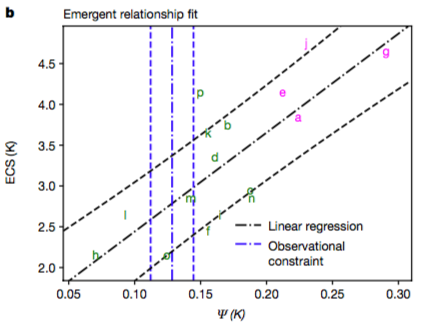
And more recently, Tapio Schneider has posted an article arguing that Cox et al underestimated their uncertainties. Unfortunately, he does this via an analysis of his own work that certainly does underestimate uncertainties, but which does not (I believe) accurately represent the Cox et al work. Here’s the Cox et al figure again, and below it another regression analysis of different data from Schneider’s blog.


It’s clear at a glance that the uncertainty bounds on the Cox et al regression basically include most of the models whereas the uncertainty bounds of Schneider exclude the vast majority of his (I’m talking about the black dashed lines in both plots). I think the simple error here is that Schneider is considering only the uncertainty on the regression line itself whereas Cox is considering the predictive uncertainty of the regression relationship. The theoretical basis for most of the emergent constraint work is that reality can be considered to be "like" one of the models in the sense of satisfying the regression relationship that the models exhibit, ie it follows on naturally from the statistically indistinguishable paradigm for ensemble interpretation (I don’t preclude the possibility that there may be other ways to justify it). The intuitive idea is that reality is just like another model for which we can observe the variable on the x-axis (albeit typically with some non-negligible uncertainty) and want to predict the corresponding variable on the y-axis. So the location of reality along the x-axis is constrained by our observations of the climate system, and it is likely to be a similar distance from the regression line as the models themselves are.
Schneider then compares his interpretation of the emergent constraint method with model weighting, this being a fairly standard Bayesian approach. We also did this in our LGM paper, though we did the regression method properly so the differences were less marked. I always meant to go back and explore the ideas underlying the two approaches in more detail, but I believe that the main practical difference is that the Bayesian weighting approach is using the models themselves as a prior whereas the regression is implicitly using a uniform prior on the unknown. The regression has the ability to extrapolate beyond the model range and also can be used more readily when there is a very small number of models, as is typically the case in paleo research.
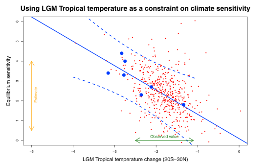
Here’s our own example from the paper which attempts to use tropical temperature at the Last Glacial Maximum as a constraint on the equilibrium sensitivity.

The models are the big blue dots (yes, only 7 of them, hence the large uncertainty in the regression). I used the random sampling (red dots) to generate the pdf for sensitivity, by first sampling from the pdf for tropical temperature and then for each dot sampling from the regression prediction. The broad scatter of the red dots is due to using t-distributions which I think is necessary due to the small number of models involved (eg even the uncertainty on the tropical temp constraint is a t-distribution as it was estimated by a leave-one-out cross validation process). But this is perhaps a bit of a fine detail on the overall picture. It is often not clear exactly how other authors have approached this and to be fair it probably matters less when considering modern constraints when data are generally more precise and ensemble sizes are rather larger.
We also did the Bayesian model weighting in this paper, but with only 7 models the result is a bit unsatisfactory. However the main reason we didn’t like it for that work is that by using the models as a prior, it already constrains the sensitivity substantially! Whereas if the observations of LGM cooling had been outside the model range, the regression would have been able to extrapolate as necessary.

Here’s the weighting approach applied to the same question, with the blue dots marking the models, the green curve is the prior pdf (equal weighting on the models) and the thick red is the posterior which is the weighted sum of the thinner red curves. Each model has to be dressed up in a rather fat gaussian kernel (standard techniques exist to choose an appropriate width) to make an acceptably smooth shape. It’s different from the regression-based answer, but not radically so, and the difference can for the most part be attributed to the different prior.
Having said all that, I’m not uncritically a fan of the Cox et al work and result, a point that I’ll address in a subsequent post. But I thought I should point out that at least these two criticisms of Schneider and Benestad seem basically unfounded and unfair.
No comments:
Post a Comment