No comment necessary

 

Chess

Many years ago, I played chess as a schoolboy. Not all that brilliantly, but good enough for the school team which played in various competitions. This fell by the wayside when I went to university, and I'd never had the time or energy to re-start though kept on playing against my uncle when we met. A couple of years ago during covid lockdowns I started playing on-line on chess.com, and then more recently someone started a chess club in Settle where a small bunch of us have been playing fairly informal and quick games. Last weekend was my first proper over-the-board competition, at the very conveniently located Ilkley Chess Festival. I'd naively assumed this would be a local event for local people, but my opponents came from all over, hailing from Portsmouth, Nottingham, Shrewsbury, and even Scarborough. There were also some Scots on the entry list that I didn't meet.

I've blogged the event on the chess.com site (here and here) as that allows for embedding of games. Spoiler alert: after losing the first game, I won the next 4, ending in 4th place. In the “Intermediate” section, which means under-1750 rated. (I don't have a current rating for OTB chess, so had to guess which section to enter. At school I was about 1450.)

Someone was taking pictures, so here is a picture of the main hall:

and here I am, about to win my 3rd game:

BlueSkiesResearch.org.uk: EGU 2022 – how cold was the LGM (again)?

I haven’t blogged in ages but have actually done a bit of work. Specifically, I eventually wrote up my new reconstruction of the Last Glacial Maximum. We did this back in 2012/3 (see here) but since then there have been lots more model simulations, and then in 2020 Jessica Tierney published a new compilation and analysis of sea surface temperature proxy data. She also produced her own estimate of the LGM temperature anomaly based on this data set, coming up with -6.1±0.4C which seemed both very cold and very precise compared to our own previous estimate of -4.0±0.8C (both ranges at 95% probability).

We thought there were quite possibly some problems with her result, but weren’t a priori sure how important a factor this might have been, so that was an extra motivation to revisit our own work.

It took a while, mostly because I was trying to incrementally improve our previous method (multivariate pattern scaling) and it took a long time to get round to realising that what I really wanted was an Ensemble Kalman Filter, which is what Tierney et al (TEA) had already used. However, they used an ensemble made by sampling internal variability of a single model (CESM1-2) and a few different sets of boundary conditions (18ka and 21ka for LGM, 0 and 3ka for the pre-industrial), whereas I’m using the PMIP meta-ensemble of PMIP2, PMIP3, and PMIP4 models.

OK, being honest, that was part of the reason, the other part was general procrastination and laziness. Once I could see where it was going, tidying up the details for publication was a bit boring. But it got done, and the paper is currently in review at CPD. Our new headline result is -4.5±1.7C, so slightly colder and much more uncertain than our previous result, but nowhere near as cold as TEA.

I submitted an abstract for the EGU meeting which is on again right now. It’s fully blended in-person and on-line now, which is a fabulous step forwards that I’ve been agitating for from the sidelines for a while. They used to say it was impossible, but covid forced their hand somewhat with two years of virtual meetings, and now they have worked out how to blend it. A few teething niggles but it’s working pretty well, at least for us as virtual attendees. Talks are very short so rather than go over the whole reconstruction again (I’ve presented early versions previously) I focussed just on one question: why is our result so different from Tierney et al? While I hadn’t set out specifically to critique that work, the reviewers seemed keen to explore, so I’ve recently done a bit more digging into our result. My presentation can be found via this link, I think.

One might assume a major reason might be that the new TEA proxy data set was substantially colder than what went before, but we didn’t find that to be the case. In fact many of the gridded data points coincide physically with the MARGO SST data set which we had previously used, and the average value over these locations was only 0.3C colder in TEA than MARGO (though there was a substantial RMS difference between the points, which is interesting in itself as it suggests that these temperature estimates may still be rather uncertain). A modest cooling of 0.3 in the mean for these SST points might be expected to translate to about 0.5 or so for surface air temperature globally, not close to to the 2.1C difference seen between our 2013 result and their 2020 paper. Also, our results are very similar when we switch between using MARGO and TEA and both together. So, we don’t believe the new TEA data are substantially different from what went before.

What is really different between TEA and our new work is the priors we used.

Here is a figure summarising our main analysis, which follows the Ensemble Kalman Filter approach, which means we have a prior ensemble of model simulations (lower blue dots, summarised in the blue gaussian curve above) each of which is updated by nudging towards observations, generating the posterior ensemble of upper red dots and red curve. I’ve highlighted one model in green, which is CESM1-2. Under this plot I have pasted bits of a figure from Tierney et al which shows their prior and posterior 95% ranges. I lined up the scales carefully. You can see that the middle of their ensembles, which are entirely based on CESM1-2, are really quite close to what we get with the CESM1-2 model (the big dots in their ranges are the median of their distributions, which obviously aren’t quite gaussian). Their calculation isn’t identical to what we get with CESM1-2, because it’s a different model simulation, with different forcing, we are using different data and there are various other differences in the details of our calculation. But it’s close.

Here is a terrible animated gif. It isn’t that fuzzy in the full presentation. What it shows is the latitudinal temperatures (anomalies relative to pre-industrial) of our posterior ensemble of reconstructions (thin black lines, thick line showing the mean), with the CESM-derived member highlighted in green, and Tierney et al’s mean estimate added in purple. The structural similarity between those two lines is striking.

A simple calculation also shows that the global temperature field of our CESM-derived sample is closer to their mean in the RMS difference sense, than any other of our ensemble members. Clearly, there’s a strong imprint of the underlying model even after the nudge towards the data sets.

So, this is why we think their result is largely down to their choice of prior. While we have a solution that looks like their mean estimate, this lies close to the edge of our range. The reason they don’t have any solutions that look like the bulk of our results is simply that they excluded them a priori. It’s nothing to do with their new data or their analysis method.

We’ve been warning against the use of single model ensembles to represent uncertainty in climate change for a full decade now, it’s disappointing that the message doesn’t seem to have got through.

Marmalade Training Camp

A trip to Scotland last weekend to learn the ancient art of Victorian Marmalade Making from marmalade sensei, the Mother in Law. It turned our to be less art and more chemistry!  I still don't quite understand how it worked, but it did. Maybe it is actually magic. It was great weather for the project; continuous rain for 3 days. 

Step 1. Get Seville oranges, and the same mass of lime and lemons. These kind of oranges are mostly pith and pips, taste very bitter, and can only be found in January, although not only in Scotland. Wash and remove the ends, and any nasty ones.

 

 

Step 2. Juice fruits! An acceptable diversion from Victorian tradition is to use an electric juicer. The juice goes into the juice pot, the pith and pips into the pith and pits pot, and the shells of rind go to the slicer. The slicer is a large heavy metal thing that clamps to the table, a handle is turned and sliced peel comes out of the bottom. A non-Victorian alternative to the slicer is unknown.

Step 3. Add water to the pith and pips bowl and to the rind. pints of water = 1.1 x weight of fruit in lbs, with about 0.1 going into the pith.

Step 4. Soaking the fruit is neither here not there as far as the chemistry/magic is concerned, apparently. But by now you will be tired, so you can take a break ... overnight if you like.

Don't forget your cat!

Step 5. Find cauldron! Put rind-marinade into cauldron.

Step 6. Manufacture a bag from cloth and string that contains the pith and pips, and suspend in cauldron. This bag contains the magical carbohydrate pectin which is required to make the marmalade set. Bring to boil and cook for an hour (the internet suggests 2-3 hours for bright, tender marmalade. The internet might be wrong.). Apparently the acid from the fruit helps get the pectin out, but I don't understand this, becuase the juice is not yet added at this stage.

Step 7. Turn off the heat. Extract bag from cauldron and squeeze it hard to get out all the pectin. 

Step 8. Add juice.

Step 9. Add sugar

Step 10. Add more sugar

Steps 11-13. Add yet more sugar. About 1.6x weight of fruit in total!!!!

Step 14. Bring slowly to a rolling boil. 

 


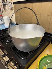
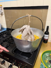
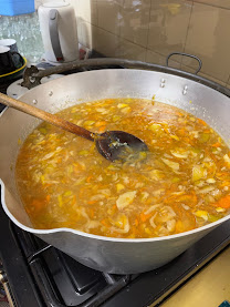
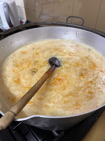
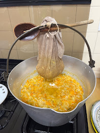
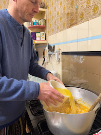
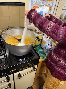
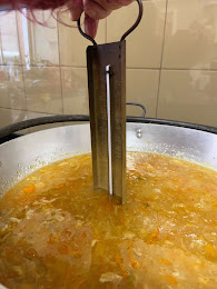
Step 15. Excitedly test every 5 seconds to see if it is done yet. It is done when it sets. This is the magic/chemistry bit. Pectin and acid and heated up sugar and do something or other that makes - jelly. But this isn't the same as caramalisation that you use to make toffee, which is more like burning sugar. In fact you want as little caramalisation as possible, because marmalade shouldn't taste like toffee. This is why the internet says boil for 15-20mins. The internet also says too much boiling at this stage make the rind tough. It was more like an hour for us, but our marmalade is still pretty and the rind very nice. Maybe internet people want the rind to melt in their mouths or something weird?

Anyway, you can test by cooling a small spoonful on a plate and when it starts to set it is done, or use a Victorian thermometer. Not sure what the markings on the thermometer engraved by ancestors mean, but when the brass holder gets all sticky with globs of marmalade, it is done.

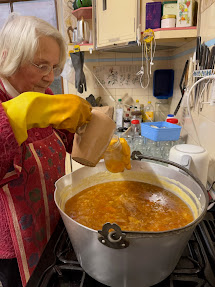
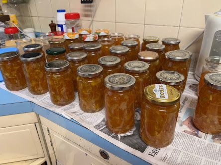
Step 16. Remove from heat and quickly fill up all your jars (which, hopefully, appear beside you by magic) and screw the lids on ASAP.  

 

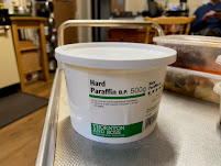
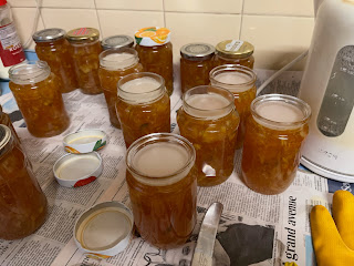
Optional Step. Next day, if some of your jars are not screw top, or they are screw top but the button on the lid didn't go down as the marmalade cooled, or you don't have lids... melt paraffin wax (in a jug in boiling water) and pour over the top and slap on some kind of lid! Marmalade will stay good for ... 3 years or so?

Step 17. Eat. Yum yum!